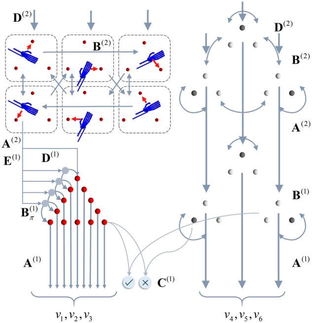
Figure 3.

Discrete generative model for movement planning. This schematic illustrates the hierarchical discrete state-space generative model that sits above the continuous model shown in Fig. 1. This model generates the hidden causes (v) that are the (imaginary) attracting points and the target locations from the perspective of the continuous model, which effectively induce movement. The discrete (categorical) causes that generate these come in two forms: the alternative attracting points (red spheres) that act as equilibrium points, and which of the three possible target locations is currently specified. These causes are themselves generated by states at a higher level. At the highest level (upper left) we have a set of alternative combinations of trajectories. Each of these is defined in terms of which vertex of a triangle (i.e. target location) is at the start and end of that trajectory. There are three configurations not shown that represent a single vertex of the triangle being the start and end of a trajectory (i.e. a static ‘trajectory’). In addition, the higher level includes a replica of the three possible target states (upper right). However, while these are considered static at the timescale of the lower level, the slower dynamics of the higher level allow this to change over time. The key distinction here is the absence of arrows between alternative target configurations at the first level. The C-vector represents the statistics of a prior belief that policies will lead to correct outcomes (i.e. hand and target location match). This ensures sequences of actions that lead to the realization of this goal are more plausible than those that do not. The arrows within a level indicate the allowed transitions (encoded by B) between these configurations. The arrows between levels show the generation of lower level variables by higher level variables. This rests upon generation of a discrete outcome via A⁽²⁾, which is then used to generate policies [via E⁽¹⁾] or initial states [via D⁽¹⁾]. The role of D⁽²⁾is to provide a prior belief about the initial states at the higher level. Note that, if we were to extend this model to include further levels, this would also become an empirical prior, recapitulating the role of D⁽¹⁾. However, given that Level 2 is the highest level considered here, D⁽²⁾is simply a vector of prior probabilities. This says that the target states may be in any initial configuration with equal probability and that the initial state probability is equally distributed among any of the trajectories that start at the lower-right target.