Figure 8:

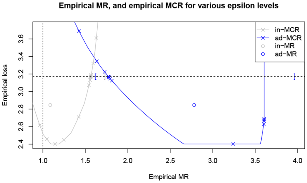
Empirical MR and MCR for Broward County criminal records data set - For any prediction model f, the y-axis shows empirical loss $({\widehat{e}}_{\mathrm{stnd}}(f))$ and the x-axis shows empirical reliance $(\widehat{MR}(f))$ on each covariate subset. Null reliance (MR equal to 1.0) is marked by the vertical dotted line. Reliances on different covariate subsets are marked by color (“admissible” = blue; “inadmissible” = gray). For example, model reliance values for f_ref are shown by the two circular points, one for “admissible” variables and one for “inadmissible” variables. MCR for different values of ϵ can be represented as boundaries on this coordinate space. To this end, for each covariate subset, we compute conservative boundary functions (shown as solid lines, or “bowls”) guaranteed to contain all models in the class (see Section 6). Specifically, all models in $f\in {\mathcal{F}}_{D,r_k}$ are guaranteed to have an empirical loss $({\widehat{e}}_{\mathrm{stnd}}(f))$ and empirical MR value $(\widehat{MR}(f))$ for “inadmissible variables” corresponding to a point within the gray bowl. Likewise, all models in ${\mathcal{F}}_{D,r_k}$ are guaranteed to have an empirical loss and empirical MR value for “admissible variables” corresponding to a point within the blue bowl. Points shown as “×” represent additional models in ${\mathcal{F}}_{D,r_k}$ discovered during our computational procedure, and thus show where the “bowl” boundary is tight. The goal of our computation procedure (see Section 6) is to tighten the boundary as much as possible near the ϵ value of interest, shown by the dashed horizontal line above. This dashed line has a y-intercept equal to the loss of the reference model plus the ϵ value of interest. Bootstrap CIs for MCR₋(ϵ) and MCR₊(ϵ) are marked by brackets.