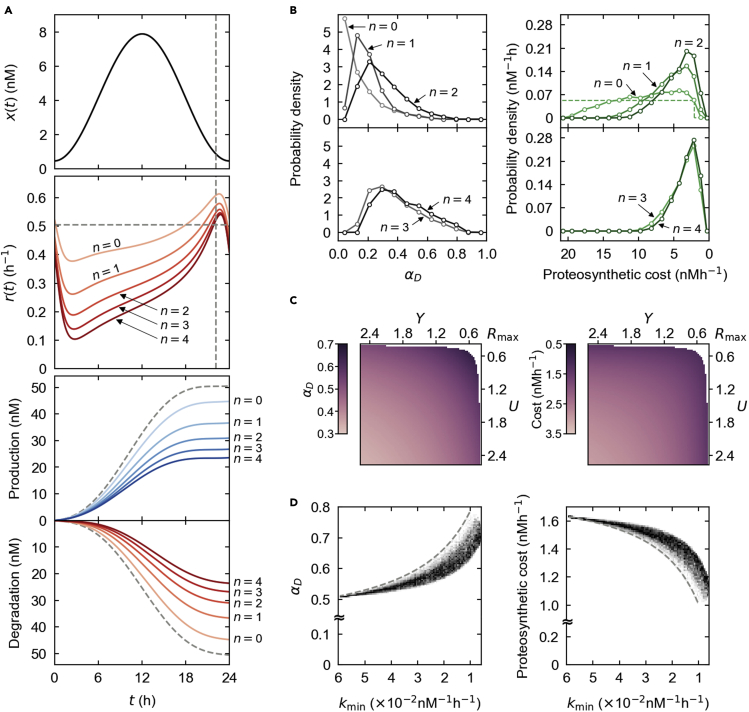
Figure 3.

Phospho-dependent degradation simulation with steady proteolytic mediators

$n$ denotes the number of phosphorylation events required for protein ubiquitination. $n=0$ corresponds to phospho-independent ubiquitination.

(A) Maintaining the protein profile $x\left(t\right)$ and model parameters in Figure 2A, we increased $n$ and simulated the degradation rate $r\left(t\right)$ for each $n$ (solid lines in the center panel). The bottom panel shows the total protein amount produced (bluish solid line) or degraded (reddish solid line) over time for each $n$. In the top and center panels, horizontal and vertical dashed lines are the same in Figure 2A with a constant degradation rate. The dashed lines in the bottom panel correspond to this constant degradation-rate case.

(B) Given the protein profile $x\left(t\right)$ in (A), we computed the probability distributions of ${\alpha }_D$ and a proteosynthetic cost for each $n$ (solid lines) over physiologically relevant parameter ranges in Table S1. The dashed line in the right upper panel corresponds to a constant degradation-rate case.

(C) When $n=1$, ${\alpha }_D$ and proteosynthetic costs are shown with varying kinase ($\propto Y$) and ubiquitin ligase ($\propto U$) concentrations, while the other parameters and $x\left(t\right)$ are fixed as (A). The top-right corner of each plot corresponds to $Y=U=R_{\text{max}}$. Biologically infeasible regimes are not plotted here (STAR Methods, computational modeling of phosphorylation-dependent protein ubiquitination; see also Figure S3).

(D) $k_{\text{min}}$ denotes the lowest binding rate of a kinase across phosphosites of a target protein. When $n=3$, the density plot of varying $k_{\text{min}}$ and the corresponding ${\alpha }_D$ was obtained over randomly sampled kinase binding rates from physiologically relevant ranges in Table S1 (the other parameters and $x\left(t\right)$ were fixed as in (A)). Likewise, the density plot of varying $k_{\text{min}}$ and the corresponding costs was obtained. The dashed lines indicate the results of the identical binding rates across the phosphosites. Figure S4 provides additional information. For visual guidance, the costs, $Y$, and $U$ in (B, C) and $k_{\text{min}}$ in (D) are arranged in the descending order. For notations here, refer to STAR Methods, computational modeling of protein ubiquitination without depending on other PTMs and computational modeling of phosphorylation-dependent protein ubiquitination. The models in (A–D) consist of (Equation 6), (Equation 7), (Equation 8), (Equation 9), (Equation 10) and (Equation 19), (Equation 20), (Equation 21), (Equation 22), (Equation 23), (Equation 24), (Equation 25), (Equation 26) in STAR Methods, computational modeling of protein ubiquitination without depending on other PTMs and computational modeling of phosphorylation-dependent protein ubiquitination with the following parameter conditions: $y=152.7$ nM (A, D), $z=0$, $k=k_1=k_2=k_3=k_4=0.013$ nM⁻¹h⁻¹ (A, C), and $k_1=k_2=k_3=k_4$ (B). The other parameters are the same as in Figure 2.