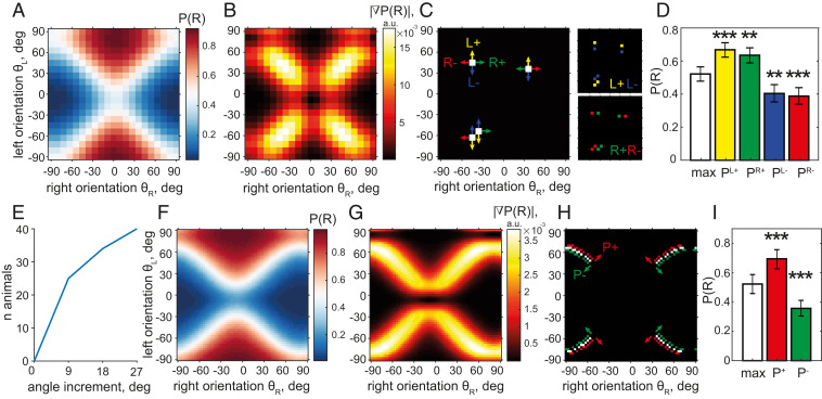
Fig. 3.

Mice reach a typical orientation acuity of 9°. (A–D) Steps of acuity analysis for an example animal. (A) P(R) model surface of an example mouse. (B) |∇P(R)| absolute value of the gradient of P(R) surface in A. (C) Four stimulus conditions (white) with |∇P(R)| in the top 5% of values and P(R) close to chance level (0.48 < P(R) < 0.52). Arrows of the same color show angle change yielding one group of neighboring conditions: P^L+ (yellow; L+ for left stimulus change that increases P(R)), P^R+ (green), P^L− (blue), P^R− (red). Insets (Right) show these conditions in the stimulus space. (D) Pooled P(R) in maximum gradient conditions (white), P^0.5 = 0.52 ± 0.04, differs from P(R) in the four neighboring conditions P^L+ = 0.67 ± 0.04, p < 2.5 $·$ 10⁻⁴ (yellow), P^R+ = 0.63 ± 0.05, p < 2.5 $·$ 10⁻³ (green), P^L− = 0.40 ± 0.05, p < 2.5 $·$ 10⁻³ (blue), P^R− = 0.39 ± 0.05, p < 2.5 $·$ 10⁻⁴ (red) (binomial CIs, χ² test, df = 1, n = 4 comparisons). (E) Population summary of analysis in A through D: cumulative number of animals for which at least one direction of angle change gives a P(R) significantly different from P^0.5 as a function of angle change magnitude. (F and G) Similar to A and B for an animal trained with 3° angle binning. (H) Maximum gradient conditions (white, same criteria as in C) and neighboring conditions obtained by changing both angles by ±3° in the direction of P(R) increase (P⁺, red) and decrease (P⁻, green). (I) Pooled P(R) in three groups highlighted in H: P^0.5 = 0.52 ± 0.04, P⁺ = 0.69 ± 0.07 (red), P⁻ = 0.36 ± 0.05 (green), both different from P^0.5 with p < 0.0005 (χ² test, df = 1; n = 2 comparisons).