Detecting Spatial Clusters of Coronavirus Infection Across London During the Second Wave

Abstract

The identification of seriously infected areas across a city, region, or country can inform policies and assist in resources allocation. Concentration of coronavirus infection can be identified through applying cluster detection methods to coronavirus cases over space. To enhance the identification of seriously infected areas by relevant studies, this study focused on coronavirus infection by small area across a city during the second wave. Specifically, we firstly explored spatiotemporal patterns of new coronavirus cases. Subsequently, we detected spatial clusters of new coronavirus cases by small area. Empirically, we used the London-wide small-area coronavirus infection data aggregately collected. Methodologically, we applied a fast Bayesian model-based detection method newly developed to new coronavirus cases by small area. As empirical evidence on the association of socioeconomic factors and coronavirus spread have been found, spatial patterns of coronavirus infection are arguably associated with socioeconomic and built environmental characteristics. Therefore, we further investigated the socioeconomic and built environmental characteristics of the clusters detected. As a result, the most significant clusters of new cases during the second wave are likely to occur around the airports. And, lower income or lower healthcare accessibility is associated with concentration of coronavirus infection across London.

Introduction

To contain the spread of coronavirus, governments implemented stay-at-home policies and social distancing measures. The closure of public places (e.g., pubs, bars, schools, etc.) and working from home prevent the spread of coronavirus among people. The identification of seriously infected areas across a city, region, or country can inform policies and assist in resources allocation. Concentration of Coronavirus infection can be identified through applying cluster detection methods to coronavirus cases over space. With the outbreak of global coronavirus pandemic, georeferenced coronavirus cases are being reported on a regular basis. To protect patient privacy, coronavirus cases are not released at the individual level. Instead, coronavirus cases are aggregated into areal units (e.g., neighborhoods/districts, towns/cities, provinces/states, countries, etc.) before being released. Recently, aggregate-level coronavirus cases by small areas are available in some countries or regions. Therefore, small-area coronavirus cases enable researchers to better explore spatial patterns of coronavirus infection and model spread of coronavirus over space and time. On the one hand, some studies performed spatial analysis of coronavirus cases across a country (e.g., Adekunle et al., 2020; Guliyev, 2020; Huang et al., 2020; Mollalo et al., 2020). They explored spatial variations of coronavirus infection rate in relation to socioeconomic and environmental factors across China (e.g., Guliyev, 2020; Huang et al., 2020), United States (e.g., Mollalo et al., 2020), and Africa (e.g., Adekunle et al., 2020). And, city-wide studies of coronavirus cases and deaths by small areas have been conducted as well (e.g., Cordes & Castro, 2020; Harris, 2020). On the other hand, some scholars modelled the dynamic spread of coronavirus according to travel patterns of people across China (Zheng et al., 2020), Italy (Gatto et al., 2020), and U.S. (Velásquez & Lara, 2020). As most of the relevant studies used the coronavirus case data collected between February and April when mass testing was not available, their findings are of some potential bias.

Moreover, the identification of areas seriously infected by coronavirus had been conducted by some studies (Desjardins et al., 2020; Hohl et al., 2020). Hohl et al. (2020) and Desjardins et al. (2020) had applied a spatio-temporal cluster detection method (i.e., Kulldorff’s prospective space–time scan statistic) to county-level coronavirus infection across U.S. To enhance the identification of seriously infected areas, we further focused on coronavirus infection by small area across a city during the second wave. Specifically, we firstly explored spatiotemporal patterns of new coronavirus cases. Subsequently, we detected spatial clusters of new coronavirus cases by small area. Empirically, we used the London-wide small-area coronavirus infection data aggregately collected. And, the data collected since June is of higher quality than those collected before June. Since mass testing is available for London since June, number of confirmed cases after June is more reliable than that before June. Methodologically, we applied a fast Bayesian model-based detection method newly developed (Gómez-Rubio et al., 2018) to new coronavirus cases by small area due to its advantages: mode-based approach accounting for covariates and the application of a fast approximation method (integrated nested Laplace approximation) instead of conventional one (Markov chain Monte Carlo methods). Gómez-Rubio et al. (2018) extend previous work (e.g., Jung, 2009) to cope with new problems and provide a new way of assessing cluster significance and importance by means of a more general model selection criteria. As empirical evidence on the association of socioeconomic factors and coronavirus spread have been found (e.g., Adekunle et al., 2020; Cordes & Castro, 2020), we could speculate that spatial clusters of coronavirus infection might be associated with socioeconomic and built environmental characteristics. Therefore, we further investigated the socioeconomic and built environmental characteristics of the clusters detected. Compared to relevant studies (Desjardins et al., 2020; Hohl et al., 2020), this study made new contributions as follow: (1) usage of more reliable data collected when mass testing is available; (2) applying a new and faster cluster detection method which can further incorporate covariates into the cluster detection; and (3) a city-wide study of coronavirus infection by small area.

Materials and Methods

Research Data

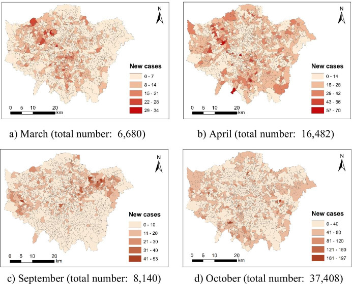
The coronavirus case count by small area is available for the UK (https://coronavirus.data.gov.uk/details/cases). The data offer monthly number of new coronavirus cases by Middle Layer Super Output Areas (MSOAs). Figure 1 maps 4-month new coronavirus cases across London at the Middle Layer Super Output Area (MSOA) level. Besides, there are 983 MSOAs across London. Total number of new coronavirus cases in London is 2004, 8140, 37,408 and 74,975 for March, April, September and October respectively. We further used the Gini coefficient to measure spatial inequality in MSOA-level new case count. Accordingly, the population-weighted Gini coefficient values of MSOA-level new case count are 0.402, 0.319, 0.455, and 0.251 for March, April, September and October respectively. Since September has the highest Gini coefficient value, new coronavirus cases are most likely to cluster around some specific areas.

Fig. 1.

New coronavirus cases across London at the Middle Layer Super Output Area (MSOA) level (March, April, September and October in 2020)

In this study, the latest demographic data by MSOA are used as covariates in the cluster detection. Specifically, population by MSOA is available for 2019 (https://www.ons.gov.uk/peoplepopulationandcommunity/populationandmigration/populationestimates/datasets/middlesuperoutputareamidyearpopulationestimates), and annual household income by MSOA is available for 2015/2016 (https://data.london.gov.uk/dataset/ons-model-based-income-estimates--msoa). The locations of hospitals, police stations and schools are acquired from the Ordnance Survey (https://www.ordnancesurvey.co.uk/business-government/products/points-of-interest); while the land use data for 2018 was downloaded from the Copernicus (https://land.copernicus.eu/local/urban-atlas).

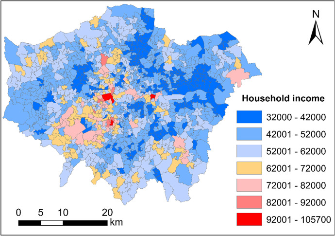
Figure 2 maps 2015/2016 annual household income (unit: British Pound) across London at the Middle Layer Super Output Area (MSOA) level.

Fig. 2.

Annual household income (unit: British Pound) across London at the Middle Layer Super Output Area (MSOA) level (2015/2016)

Exploring Spatiotemporal Patterns of Coronavirus Infection

Exploring Spatial and Temporal Variations of Coronavirus Infection

In this study, we first explored spatial and temporal variations of coronavirus infection respectively.

Exploring Spatial Shift of Highly Infected Areas

In this study, we subsequently explored spatial shift of highly infected areas by investigating local spatial association of coronavirus infection rate before the wave and coronavirus infection rate during the wave. Accordingly, bivariate local Moran’s I test is used to quantify the local spatial association between two variables. Specifically, a positive association (a positive Moran’s I value) means high (low) values of one variable is surrounded by high (low) values of the other variable; whilst a negative association (a negative Moran’s I value) means high (low) values of one variable is surrounded by low (high) values of the other variable. Besides, the bivariate local Moran’s I testing was implemented in GeoDa (http://geodacenter.github.io/index.html).

Detecting Spatial Clusters of Coronavirus Infection

Fast Bayesian Model-Based Cluster Detection

Based on the model-based approaches of Jung (2009) for the detection of spatial disease clusters to space and time (Gómez-Rubio et al., 2019), Gómez-Rubio et al. (2018) propose a new approach that uses dummy variables in a regression model to group regions into clusters. The importance of the clusters is then assessed based on a likelihood calculation that measures the extent to which the clusters capture the variability in the outcome (Gómez-Rubio et al., 2018). To address a huge computational burden due to the usage of Bayesian hierarchical models fit by means of Markov chain Monte Carlo (MCMC) methods, Gómez-Rubio et al. (2018) use a fast approximation method (integrated nested Laplace approximation) proposed by Rue et al. (2009) to fit the model, and provide a reasonable estimate of the coefficient of the cluster variables and compute the deviance information criterion (DIC) in model selection. Theoretically, the problem of cluster detection is regarded as a problem of variable selection, where covariates include a number of dummy variables that represent all possible clusters (Gómez-Rubio et al., 2018). Hence, when fitting individual model to test for different clusters, this approach, based on integrated nested Laplace approximation (INLA), will be faster than fitting the same models with MCMC (Gómez-Rubio et al., 2018).

For the sake of brevity, we present the model as follows (Gómez-Rubio et al., 2019): “

$$\log ({\mu }_{i,t})=\log (E_{i,t})+{\gamma }_j{c}_{i,t}^{(j)}$$ 1

where μ_i,t is the mean of area i at time t, and E_i,t is the expected number of cases in area i at time t. $c_{i,t}^{(j)}$ is a cluster dummy variable for spatio-temporal cluster j, and ${\gamma }_j$ is the coefficient of the cluster dummy variable.” Moreover, the expected number of cases E_i,t is computed through fitting a Poisson regression (generalised linear model) with offset log(E_i,t) on the covariates (Gómez-Rubio et al., 2018).

Covariates

Table 1 lists the covariates at the MSOA level, including socioeconomic characteristics (i.e., income, hospital accessibility, police station accessibility, school accessibility, population density) and built environment characteristics (i.e., land use composition and land use mix). Since a large portion of MSOAs have no hospitals and police stations, this study selected distance-based measures instead of density-based or count-based measures to quantify accessibility to hospital or police station. Table 2 shows the statistical description for all the covariates in this study.

Table 1.

Covariates considered in this study

Type	Variable	Full name
Socioeconomic characteristics	AHI	Annual household income (unit: 1,000 £)
	Dis_Hos	Distance to nearest hospital (unit: km)
	Dis_PS	Distance to nearest police station (unit: km)
	Den_Sch	Density of schools (unit: number of schools per km2)
	Den_Pop	Density of population (unit: 1000 persons per km2)
Built environmental characteristics	Res_Per	Residential percent (%)
	CIT_Per	Commercial, industrial & transportation percent (%)
	Rec_Per	Recreational percent (%)
	LUX	Land use mix (Entropy index)

Table 2.

Statistical description for all the covariates in this study

Variable	Mean	SD
AHI	51.38	10.77
Dis_Hos	1.69	1.01
Dis_PS	2	1.34
Den_Sch	2.83	2.65
Den_Pop	9.03	5.33
Res_Per	57.99	17.51
CIT_Per	22.66	11.59
Rec_Per	14.7	13.53
LUX	4.15	1.1

Implementation

In this study, the cluster detection was implementable in R. Specifically, the model-based cluster detection method used is supported by an R package named “DClusterm” (Gómez-Rubio et al., 2019).

Empirical Results

Spatiotemporal Patterns of Coronavirus Infection

We first explored spatiotemporal patterns of coronavirus infection in London.

Identifying the Second Wave

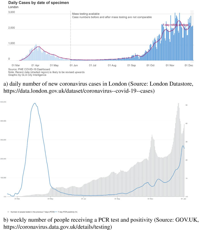
Figure 3a shows city-level daily number of new coronavirus cases in London. London is experiencing the first wave and the second wave in April and November respectively according to daily number of new cases confirmed in London. As mass testing was not available until June 2020, the number of new coronavirus cases was likely to be undercounted. At the same time, testing count during the second wave is dramatically higher than that during the first wave (see Fig. 3b). Therefore, the reported amount of new coronavirus cases during the second is more reliable than that during the first wave. From September, a number of international students who were infected arrived in London. Since most of the students live in student dormitories, coronavirus virus is likely to transmit among students in dormitories. And, students are also likely to gather in pubs and travel around the city. Not only students but also residents are at increasing risk of being infected since the start of new semester.

Fig. 3.

Coronavirus cases and tests conducted in London during 2020

Spatial Patterns of New Coronavirus Cases During the Second Wave

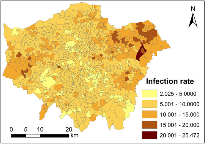
Figure 4 maps the coronavirus infection rate (unit: new cases per 1000 persons) across London at the Middle Layer Super Output Area (MSOA) level in November. The Outer London areas are more seriously infected than the Inner London areas.

Fig. 4.

Coronavirus infection rate (unit: new cases per 1000 persons) across London at the Middle Layer Super Output Area (MSOA) level during November of 2020

Spatial Shift of Highly Infected Areas

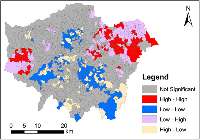
We performed the bivariate local Moran’s I test of ‘COVID-19 infection rate in October’ and ‘COVID-19 infection rate in November’. The bivariate local Moran’s I testing result is shown in Fig. 5. Figure 5 maps the clusters and outliers of ‘COVID-19 infection rate in October’ and ‘COVID-19 infection rate in November’. In Fig. 5, all the clusters and outliers are statistically significant at the 0.05 level. Clusters and outliers indicate the existence of positive and negative local spatial association respectively. Specifically, ‘High–High’ and ‘Low–Low’ represent two types of clusters; whilst ‘Low–High’ and ‘High–Low’ represent two types of outliers. In Fig. 5, ‘High–High’ means an area (MSOA) with a high value of ‘COVID-19 infection rate in October’ is surrounded by areas (MSOAs) with a high value of ‘COVID-19 infection rate in November’; ‘Low–Low’ means an area (MSOA) with a low value of ‘COVID-19 infection rate in October’ is surrounded by areas (MSOAs) with a low value of ‘COVID-19 infection rate in November’; ‘Low–High’ means an area (LAD) with a low value of ‘COVID-19 infection rate in October’ is surrounded by areas (MSOAs) with a high value of ‘COVID-19 infection rate in November’; and ‘High–Low’ means an area (MSOA) with a high value of ‘COVID-19 infection rate in October’ is surrounded by areas (MSOAs) with a low value of ‘COVID-19 infection rate in November’. Particularly, outliers indicate the shift of highly infected areas from October to November. Specifically, ‘High–Low’ areas are located around the urban centre; whilst ‘Low–High’ areas are located around the outskirts. This shows some of the highly infected areas shift from the central and southern London to the eastern and western London between October and November.

Fig. 5.

Clusters and outliers of coronavirus infection rate in October and November across London (October and November, 2020)

Cluster Detection (Spatial Clusters of New Cases)

In this subsection, we detected spatial clusters of new cases across London during the second wave (i.e., November). We applied the fast Bayesian model-based cluster detection method to the 983 observations (983 MSOAs) with no covariates and after adjusting for covariates respectively.

Cluster Detection with No Covariates

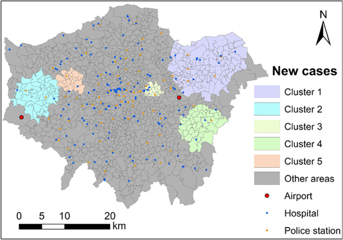
First of all, we implemented the model-based cluster detection method with no covariates. Standardised expected number of new cases E_i,t was computed fitting a Poisson regression (generalised linear model) with offset log(E_i,t) (see Eq. (1)). As a result, 24 statistically significant clusters were detected with a p-value of below 0.05. After ranking these clusters according to the DIC, top 5 clusters are list in Table 3 and mapped in Fig. 6. Those 5 clusters totally have 20% of the population of London. And those 5 clusters are all located around the Outer London rather than the Inner London (central London).

Table 3.

Statistically significant clusters of coronavirus infection

Cluster	Size	At-risk population	At-risk population percent	DIC	p-value	Risk
1	92	852,230	9.51	1086.356	< 0.001	0.470
2	38	361,260	4.03	233.220	< 0.001	0.349
3	17	172,906	1.93	177.882	< 0.001	0.429
4	34	273,618	3.05	106.227	< 0.001	0.277
5	15	140,653	1.57	32.745	< 0.001	0.219
…	…	…	…	…	…	…

Fig. 6.

Five most significant clusters of coronavirus infection across London during November of 2020

Cluster Detection After Adjusting for Covariates

Subsequently, we implemented the model-based cluster detection method after adjusting for covariates. Covariate standardised expected number of coronavirus cases E_i,t was computed fitting a Poisson regression (generalised linear model) with offset log(E_i,t) on one covariate: AHI (annual household income). The generalised linear model (GLM) estimated is shown in Table 4. Expectedly, AHI is statistically significantly and negatively associated with observed number of coronavirus cases (response); and Dis_Hos is statistically significantly and positively associated. Unexpectedly, apart from Den_Sch and LUX, the remaining covariates (i.e., Den_Pop, Res_Per, CIT_Per and Rec_Per) are statistically significantly and negatively associated with observed number of coronavirus cases.

Table 4.

Estimation results for the generalised linear model (GLM) (N = 983)

Covariate	Coefficient
Intercept	1.01 ***
AHI	− 0.011 ***
Dis_Hos	0.033 ***
Dis_PS	− 0.021 ***
Den_Sch	0.0001
Den_Pop	− 0.011 ***
Res_Per	− 0.004 ***
CIT_Per	− 0.004 ***
Rec_Per	− 0.004 ***
LUX	− 0.007 .
AIC	13,958

Significance codes: ‘***’: 0.001; ‘**’: 0.01; ‘*’: 0.05; ‘.’: 0.1; ‘ ’: 1

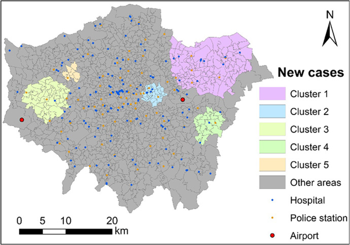
Eventually, 28 statistically significant clusters were detected with a p-value of below 0.05. After ranking these clusters according to the DIC, top 5 clusters are list in Table 5 and mapped in Fig. 7. The difference between the top 5 clusters detected with and without the covariate is not large. This means that the occurrence of those top 5 clusters is insufficiently explained by the covariates. Compared to the other clusters, Cluster 4 and Cluster 5 experience a dramatic decrease in size and at-risk population (i.e., a decrease by over 40%) before and after adjusting for covariates (see Figs. 6 and 7 as well as Tables 3 and 5). This indicates that Cluster 4 and Cluster 5 is partly attributable to the socioeconomic and built environmental characteristics.

Table 5.

Statistically significant clusters of coronavirus infection after adjusting for one covariate (i.e., annual household income)

Cluster	Size	At-risk population	At-risk population percent	DIC	p-value	Risk
1	94	878,685	9.80	729.713	< 0.001	0.376
2	27	266,431	2.97	228.369	< 0.001	0.413
3	40	365,366	4.08	110.268	< 0.001	0.237
4	18	155,709	1.74	96.783	< 0.001	0.341
5	7	69,220	0.77	19.014	< 0.001	0.229
…	…	…	…	…	…	…

Fig. 7.

Five most significant clusters of coronavirus infection after adjusting ‘annual household income’ across London during November of 2020

Discussion

London always has the highest coronavirus infection rate in the UK whilst the UK is one of the most seriously infected countries worldwide. London is densely populated and a top destination of international travellers. Particularly, after the summer most of the international students need to fly to London before going to their final destinations by train, bus, or car. Increasing coronavirus viruses were transmitted by students to London since the start of fall semester in September. This is arguably one key cause of the second wave.

The top 3 clusters are insufficiently attributable to socioeconomic and built environmental characteristics. Additionally, after comparing Figs. 1b and 7, we can find that the top 5 clusters are located around the areas that had been highly infected during the first wave (April 2020). Arguably, the top 5 clusters are partly attributable to the locals infected during the first wave. However, given the lack of individual-level coronavirus contact-tracing data it is nearly impossible to precisely assess how much contribution is made by locals or travellers.

Although clusters of coronavirus infection during the second wave are insufficiently attributable to socioeconomic characteristics, the findings in this study suggest that socioeconomically disadvantaged areas (i.e., areas with a lower income or a lower healthcare accessibility) are more likely to suffer a high risk of coronavirus or alike pandemics. Resource allocation by government should prioritise socioeconomically disadvantaged areas. And, stricter measures should be implemented in socioeconomically disadvantaged areas to reduce spatial disparities in coronavirus infection across London. Besides, effective tracking tools (e.g., coronavirus contact-tracing apps) are needed to better curb the spread of coronavirus in those areas.

Conclusion

In this study, we detected clusters of new coronavirus cases around London during the second wave. We applied a fast Bayesian model-based cluster detection method to small-area number of new cases in November. As a result, the most significant clusters of new cases during the second wave are likely to occur in low-income areas with a low level of hospital access or a low level of police station access around the airports. The empirical study suggests a policy implication that socioeconomically disadvantaged areas are more likely to suffer a high risk of coronavirus or alike pandemics. Besides, the fast Bayesian model-based detection method is efficient and robust.

However, there are some limitations in this study. Firstly, we did not undertake spatiotemporal cluster detection due to data sparsity. Secondly, we did not compare the highly infected areas between November and April when is the first wave. Since mass testing was available since June, the number of confirmed cases is not appropriately comparable between November (mass testing available) and April (mass testing unavailable). It might be of much interest to compare concentration of coronavirus infection between the two waves. Thirdly, in the explanation of the occurrence of coronavirus clusters, we take no account of mobility patterns, such as the number of daily trips or time spent out of home, due to the lack of data. Fourthly, given the lack of accurate categorisation in the POI data used, schools were not further classified into primary schools, secondary schools, universities/colleges and others. Otherwise, the association of schools and coronavirus infection might differ from primary school to university/college since the latter has a substantially higher proportion of students who had international travel. Finally, unexpectedly, this study found that all the three main land use categories (i.e., residential land, recreational land, and commercial, industrial & transportation land) are likely to curb coronavirus infection and land use mix is not statistically significantly associated with coronavirus infection.

In the future, we will improve this study by addressing those limitations. Firstly, we would undertake spatiotemporal cluster detection at a lower geography level to address the data sparsity issue. Secondly, we would compare spatial clusters of coronavirus infection between the two waves once the number of coronavirus cases before the availability of mass testing could be adjusted through some models in future. The results would be compared with those in this paper to discuss the nfluence of time gap in some data on the model estimation results. Thirdly, we would attempt to acquire mobility data from social media or mobile phone data in future. We would investigate the how mobility patterns contribute to the clusters of coronavirus infection. Fourthly, we would focus more on accessibility to university/college than accessibility to school in general once the locations of accurately categorised schools are acquirable in the future. Finally, more studies are needed to further investigate the association of land use characteristics and coronavirus infection.

Author Contributions

Conceptualization: [YS, JX, XH]; Methodology: [YS]; Formal analysis and investigation: [YS, JX, XH]; Writing—original draft preparation: [YS, JX, XH]; Writing—review and editing: [YS, JX, XH]; Resources: [YS, JX].

Funding

No funding was received.

Data Availability

Available on request.

Code Availability

Available on request.

Declarations

Conflict of interest

The authors declare that they have no conflict of interest.

Ethical Approval

Ethical approval is not required as only secondary data used in the study.

References

- Adekunle IA, Onanuga A, Wahab O, Akinola OO. Modelling spatial variations of coronavirus disease (COVID-19) in Africa. Science of The Total Environment. 2020;729:138998. doi: 10.1016/j.scitotenv.2020.138998. [DOI] [PMC free article] [PubMed] [Google Scholar]
- Cordes J, Castro MC. Spatial analysis of COVID-19 clusters and contextual factors in New York City. Spatial and Spatio-temporal Epidemiology. 2020;34:100355. doi: 10.1016/j.sste.2020.100355. [DOI] [PMC free article] [PubMed] [Google Scholar]
- Desjardins MR, Hohl A, Delmelle EM. Rapid surveillance of COVID-19 in the United States using a prospective space-time scan statistic: Detecting and evaluating emerging clusters. Applied Geography. 2020;118:102202. doi: 10.1016/j.apgeog.2020.102202. [DOI] [PMC free article] [PubMed] [Google Scholar]
- Gatto M, Bertuzzo E, Mari L, Miccoli S, Carraro L, Casagrandi R, Rinaldo A. Spread and dynamics of the COVID-19 epidemic in Italy: Effects of emergency containment measures. Proceedings of the National Academy of Sciences. 2020;117(19):10484–10491. doi: 10.1073/pnas.2004978117. [DOI] [PMC free article] [PubMed] [Google Scholar]
- Gómez-Rubio, V., Molitor, J., & Moraga, P. (2018). Fast Bayesian classification for disease mapping and the detection of disease clusters. In Quantitative methods in environmental and climate research (pp. 1–27). Springer.
- Gómez-Rubio V, Moraga P, Molitor J, Rowlingson B. DClusterm: Model-based detection of disease clusters. Journal of Statistical Software. 2019 doi: 10.18637/jss.v090.i14. [DOI] [Google Scholar]
- Guliyev H. Determining the spatial effects of COVID-19 using the spatial panel data model. Spatial Statistics. 2020;38:100443. doi: 10.1016/j.spasta.2020.100443. [DOI] [PMC free article] [PubMed] [Google Scholar]
- Harris R. Exploring the neighbourhood-level correlates of Covid-19 deaths in London using a difference across spatial boundaries method. Health & Place. 2020;66:102446. doi: 10.1016/j.healthplace.2020.102446. [DOI] [PMC free article] [PubMed] [Google Scholar]
- Hohl A, Delmelle E, Desjardins M, Lan Y. Daily surveillance of COVID-19 using the prospective space-time scan statistic in the United States. Spatial and Spatio-temporal Epidemiology. 2020;34:100354. doi: 10.1016/j.sste.2020.100354. [DOI] [PMC free article] [PubMed] [Google Scholar]
- Huang R, Liu M, Ding Y. Spatial-temporal distribution of COVID-19 in China and its prediction: A data-driven modeling analysis. The Journal of Infection in Developing Countries. 2020;14(03):246–253. doi: 10.3855/jidc.12585. [DOI] [PubMed] [Google Scholar]
- Jung I. A generalized linear models approach to spatial scan statistics for covariate adjustment. Statistics in Medicine. 2009;28(7):1131–1143. doi: 10.1002/sim.3535. [DOI] [PubMed] [Google Scholar]
- Mollalo A, Vahedi B, Rivera KM. GIS-based spatial modeling of COVID-19 incidence rate in the continental United States. Science of The Total Environment. 2020;728:138884. doi: 10.1016/j.scitotenv.2020.138884. [DOI] [PMC free article] [PubMed] [Google Scholar]
- Rue H, Martino S, Chopin N. Approximate Bayesian inference for latent Gaussian models by using integrated nested Laplace approximations. Journal of the Royal Statistical Society: Series B (Statistical Methodology) 2009;71(2):319–392. doi: 10.1111/j.1467-9868.2008.00700.x. [DOI] [Google Scholar]
- Velásquez RMA, Lara JVM. Forecast and evaluation of COVID-19 spreading in USA with Reduced-space Gaussian process regression. Chaos, Solitons & Fractals. 2020;136:109924. doi: 10.1016/j.chaos.2020.109924. [DOI] [PMC free article] [PubMed] [Google Scholar]
- Zheng R, Xu Y, Wang W, Ning G, Bi Y. Spatial transmission of COVID-19 via public and private transportation in China. Travel Medicine and Infectious Disease. 2020;34:101626. doi: 10.1016/j.tmaid.2020.101626. [DOI] [PMC free article] [PubMed] [Google Scholar]
Associated Data
This section collects any data citations, data availability statements, or supplementary materials included in this article.
Data Availability Statement