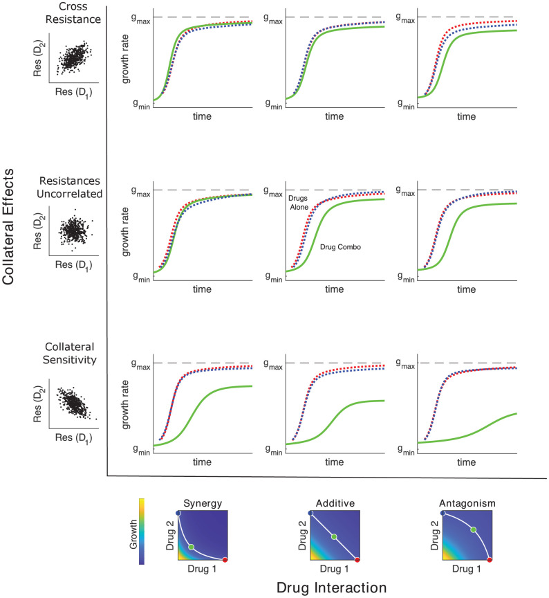
Figure 4. Adaptation depends on drug interactions and collateral effects of resistance.

Drug interactions (columns) and collateral effects (rows) modulate the rate of growth adaptation (main nine panels). Evolution takes place at one of three dosage combinations (blue, drug 2 only; cyan, drug combination; red, drug 1 only) along a contour of constant growth in the ancestral growth response surface (bottom panels). Drug interactions are characterized as synergistic (left), additive (center), or antagonistic (right) based on the curvature of the isogrowth contours. Collateral effects describe the relationship between the resistance to drug 1 and the resistance to drug 2 in an ensemble of potential mutants. These resistance levels can be positively correlated (top row, leading to collateral resistance), uncorrelated (center row), or negatively correlated (third row, leading to collateral sensitivity). Growth adaptation (main nine panels) is characterized by growth rate over time, with dashed lines representing evolution in single drugs and solid lines indicating evolution in the drug combination. In this example, response surfaces are generated with a classical pharmacodynamic model (symmetric in the two drugs) that extends Loewe additivity by including a single-drug interaction index that can be tuned to create surfaces with different combination indices (Greco et al., 1995). The initial population consists of primarily ancestral cells $(\alpha =\beta =1)$ along with a subpopulation 10⁻² mutants uniformly distributed among the different phenotypes. Scaling parameters are sampled from a bivariate normal distribution with equal variances (${\sigma }_{\alpha }={\sigma }_{\beta }$) and correlation ranging from 0.6 (top row) to −0.6 (bottom row). See also Figure 4—figure supplement 1 for gradient approximation to selection dynamics.

Figure 4—figure supplement 1. Illustration of the local growth gradient approximation to the Price equation.

(A, B) Comparison between numerical solutions to the full Price equation (dotted line), the local growth gradient approximation (solid line), and the trajectory of pure (unweighted) gradient descent (dashed line) for mean resistance evolution to two drugs ($\overline{\alpha }(t),\overline{\beta }(t)$). The dotted and solid lines are almost indistinguishable. In (A) and (B), we assume two growth landscapes respectively (drug combination 1 vs. drug combination 3, see Figure 3—figure supplement 1A, C), external concentrations $(x_0,y_0)=0.4\times (x_{max},y_{max})$, and initial trait distributions following the empirically derived (${\alpha }_i,{\beta }_i)$. The large black dot represents the initial value ($\overline{\alpha }(0),\overline{\beta }(0)$) under initial ancestor frequency of 90% and the remaining 10% spread uniformly among available mutants (denoted via the small black asterisks in the 2-D trait space). (C, D) Root mean square error between mean trait evolution calculated with the full iteration of the Price equation and the gradient approximation (for the two cases in A and B, respectively), varying ancestor initial frequency. Here for each $p\in (0.5,1)$ (the initial frequency of the ancestor subpopulation with scaling parameters $\alpha =\beta =1$), we simulated 20 stochastic realizations of the evolutionary process under drug dosage $(x_0,y_0)$, starting from different random frequencies for the remaining $1-p$ proportion of the population composed of available mutants.