Fig. 4.

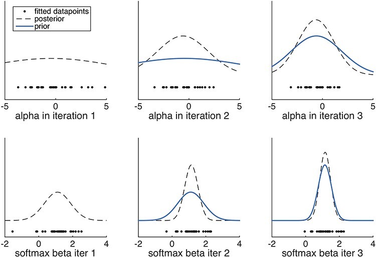
Illustration of the effects of hierarchical fitting for two parameters alpha (learning rate) and beta (softmax temperature). Left column: shown are the initial alphas and softmax betas obtained using a flat prior. The posterior obtained from the first iteration is shown in the dashed black line. Middle column: in this iteration, the posterior from iteration 1 becomes the prior (blue). This ‘pulls in’ several estimates that were previously at the more extreme ends of the range for alpha and beta. The posterior from this second iteration is sharper. Right column: Using the posterior from iteration 2 as the prior in iteration 3, there are only smaller changes in parameter estimates in this third iteration. More iterations would follow (not shown) until the algorithm converges. Note that both parameters are shown in a range between [-Inf, Inf] here. They are transformed to values between [0, 1] for alpha or positive values for beta using the transformations 1/(1 + exp(−alpha)) and exp(beta), respectively.