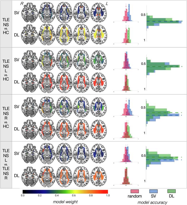
Fig. 4.

Summary of results for models based on fractional anisotropy data for patients without hippocampal sclerosis. For each of the four classifications (identified in the leftmost column), the top row shows the results for the support vector (SV) approach and the bottom row shows the results for the deep learning (DL) approach. White matter tracts are shown on axial slices from ventral to dorsal. The orientation corresponds to radiological reference (i.e., the left side of the axial slice corresponds to the right side of the brain, and vice versa). Each bundle corresponds to a region of interest (ROI) based on the Johns Hopkins University atlas colored based on the colormap at the bottom of the figure and normalized from 0 to 1, where higher values (more red regions) correspond to the most influential ROIs for that particular model. For each classification approach, a distribution of accuracies is shown to the right for permutated labels (red) or real labels (blue for SV, green for DL). The rightmost graph compares the accuracy of SV vs. DL against each other. Notice that models for which ROI weights have less variable distribution (i.e., all ROIs are relatively of equal importance for classification, as shown by a similar color range across all regions) tend to have worse performance accuracies. (For interpretation of the references to color in this figure legend, the reader is referred to the web version of this article.)