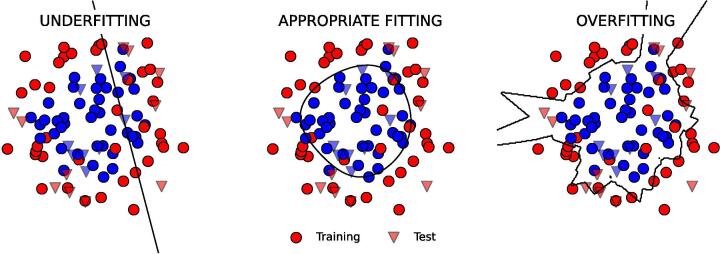
Fig. 2.

Examples of under-, appropriate and over-fitting. The input dataset consists of two classes (blue and red points) that are distributed on an inner and outer circle, respectively (with Gaussian noise) in a two dimensional feature space. Three different models are used to fit the input training set, or in other words, to find the boundary (in black) that can best separate the two classes under the model hypotheses. The training set is represented by circles, the test set by triangles. The chosen methods, Logistic Regression, Support Vector Machine with Gaussian kernel, and K-NN lead to typical over-, appropriate, and under-fitting scenarios, respectively. The code used to generate this figure is available on Github.