Figure 2.

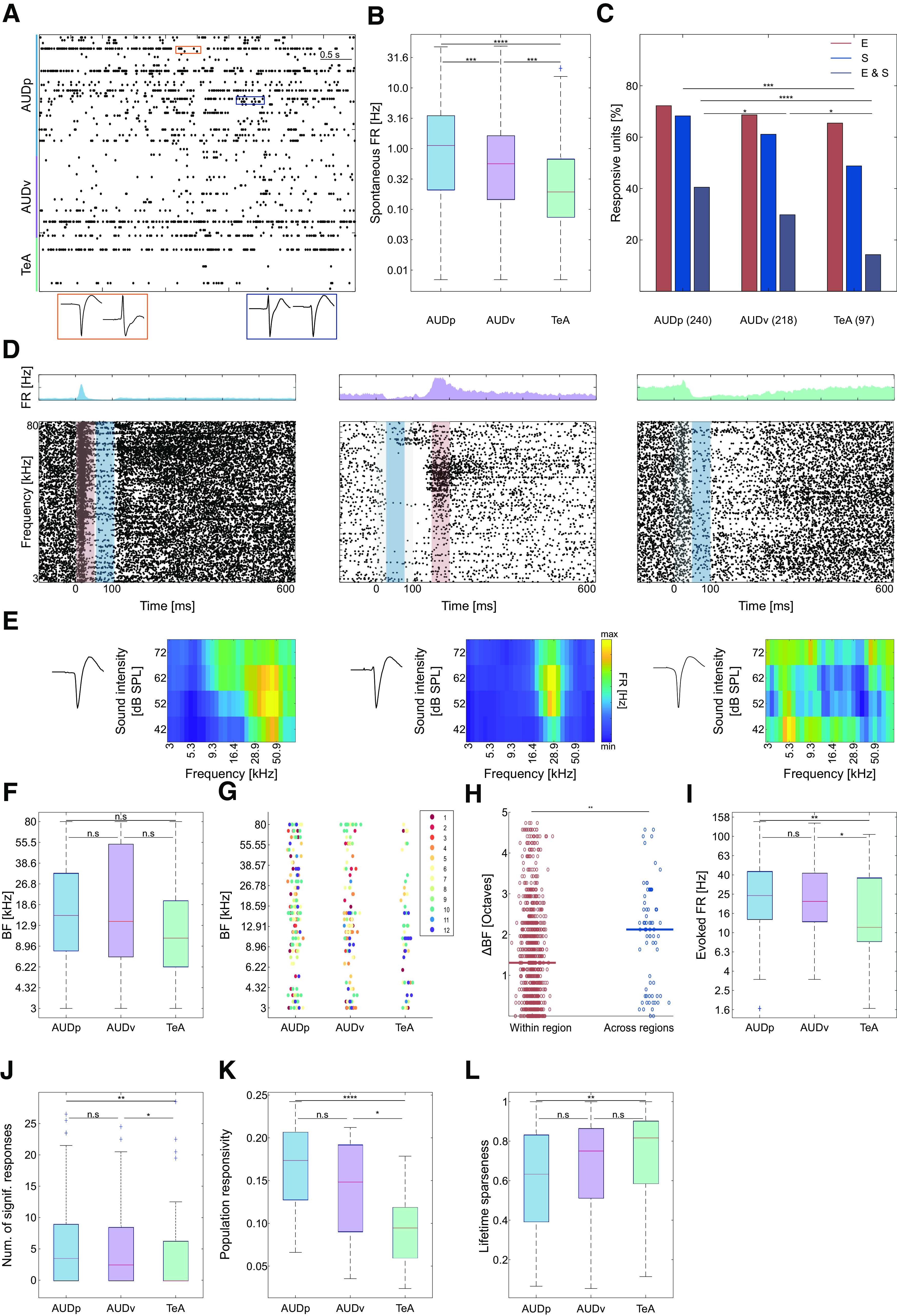
Pure tone response properties in TeA, AUDp, and AUDv. A, Raster plot showing 5 s of spontaneous activity. Color bar shows annotated regions according to channel and depth. Examples of waveforms from two pairs of SUs recorded from the same channel are shown at the bottom (orange pair, channel 173; blue pair, channel 130). B, Spontaneous FRs (log-scaled) of SUs in the three cortices [median (IQR): AUDp, 1.13 (0.21–3.48) n = 240; AUDv, 0.56 (0.14–1.63) n = 218; TeA, 0.19 (0.07–0.67) n = 97]. Spontaneous FRs decrease along the auditory D-V axis (H₍₂₎ = 35.85, p < 1e-4; Kruskal–Wallis), are highest in AUDp, and lowest in TeA (AUDp vs AUDv p = 0.003, AUDp vs TeA p < 1e-4, AUDv vs TeA p = 0.003; TK HSD test). C, Bar graph showing the distribution of response types to pure tones (E, excitatory; S, suppressive, E&S, both) in all cortical regions. Percentage computed out of all responsive units (number of SUs shown in parentheses). Excitatory responses are abundant and their fraction is maintained high in all three cortices (H₍₂₎ = 1.5, p = 0.47; Kruskal–Wallis), while abundance of suppressed units (H₍₂₎ = 10.06, p = 0.006; Kruskal–Wallis; AUDp vs AUDv, p = 0.28 n.s.; AUDp vs TeA p < 0.005; AUDv vs TeA p = 0.12 n.s.; TK HSD test) as well as units showing both response types decreases from AUDp to TeA (H₍₂₎ = 20.1, p < 1e-4; Kruskal–Wallis; AUDp vs AUDv, p = 0.048; AUDp vs TeA, p < 1e-4; AUDv vs TeA, p = 0.03 TK HSD test). D, Three examples of SU responses to pure tones recorded in AUDp (left), AUDv (center), and TeA (right). Above each raster is the unit's PSTH (scale adjusted per unit). Stimulus is presented between 0 and 100 ms (gray shaded region), and each units' maximal or minimal response window is marked by a red and/or blue bar, respectively. The units are categorized as excitatory and suppressed (left and center) and suppressed (right). E, FRAs corresponding to the three SUs shown in D. FRAs pixel values correspond to the excitatory (left and center) or suppressive (right) response window. To the left of the FRAs, spike waveform templates of the corresponding units are shown. F, SU BFs across brain regions [median (IQR): AUDp, 15.5 (8.3–32.3) kHz, n = 164 SUs; AUDv, 13.8 (7.4–53.9) kHz, n = 136 SUs; TeA, 10.4 (6.3–20.0) kHz, n = 55 SUs]. We found no effect of brain region over BF (H₍₂₎ = 3.07, p = 0.21; Kruskal–Wallis), as well as no difference between BF medians (AUDp vs AUDv, U = 2.470e4, p = 0.98 n.s.; AUDp vs TeA U = 1.875e4, p = 0.08 n.s.; AUDv vs TeA U = 1.357e4, p = 0.14 n.s.; Wilcoxon rank-sum test). G, SU BF distribution by recorded region and probe penetration. Each point represents the BF of one SU, with colors corresponding to unique probe penetrations (units sharing color were simultaneously recorded). BF distribution in all regions do not vary across penetrations (H₍₁₁₎ = 18.92, p = 0.06; Kruskal–Wallis); however, within region one, AUDv recording (#7) was biased toward high BF ranges (AUDp, H₍₁₁₎ = 9.97, p = 0.53 n.s.; AUDv, H₍₁₁₎ = 32.74, p = 0.0006; TeA, H₍₁₁₎ = 10.46, p = 0.23 n.s.; Kruskal–Wallis). H, BFs difference in octaves of adjacent SUs (⩽8 contacts apart or up to ∼80-μm distance) originating from the same or different (“within region”/“across regions”) brain regions [median (IQR): within region, 1.31 (0.49–2.29) octaves, n = 880 pairs; across regions, 2.12 (0.49–2.87), n = 69 pairs]. Transition between auditory cortices shows increased shifts in units' BFs (U = 4.110e5, p = 0.0013; Wilcoxon rank-sum test). I, Evoked FRs at BFs [median (IQR): AUDp, 24.5 (13.9–43.3) Hz, n = 164 SUs; AUDv, 21.2 (13.1–41.7) Hz, n = 136 SUs; TeA, 11.4 (8.2–37.2) Hz, n = 55 SUs]. SUs in TeA had lower FRs compared with units from both AUDp and AUDv (H₍₂₎ = 11.13, p = 0.004; Kruskal–Wallis; AUDp vs AUDv, p = 0.63 n.s.; AUDp vs TeA, p = 0.002; AUDv vs TeA, p = 0.03; TK HSD test). J, Bandwidth of SUs assessed as the number of frequencies at 62 dB SPL evoking a significant response [median (IQR): AUDp, 3.5 (0–9), n = 164 SUs; AUDv, 2.5 (0–8.5), n = 136 SUs; TeA, 0 (0–6.25), n = 55 SUs]. Bandwidth in TeA was smaller than in AUDp and AUDv (H₍₂₎ = 10.08, p = 0.006; Kruskal–Wallis; AUDp vs AUDv, p = 0.6 n.s.; AUDp vs TeA, p = 0.004; AUDv vs TeA, p = 0.04; TK HSD test). K, Population sparseness quantified as response probabilities of SUs in each region to all frequencies played at 62 dB SPL [median (IQR): AUDp, 0.17 (0.12–0.21), AUDv, 0.15 (0.09–0.19), TeA, 0.09 (0.06–0.12)]. Response probability is highest in AUDp and lowest in TeA (H₍₂₎ = 21.86 p < 1e-4; Kruskal–Wallis; AUDp vs AUDv, 0.2 n.s.; AUDp vs TeA, p < 1e-4; AUDv vs TeA, p = 0.01; TK HSD test). L, Lifetime sparseness of SUs [median (IQR): AUDp, 0.64 (0.39–0.83), AUDv, 0.75 (0.51–0.87), TeA, 0.82 (0.59–0.90)]. Sparseness was larger in TeA compared with AUDp (H₍₂₎ = 11.32, p = 0.003; Kruskal–Wallis; AUDp vs AUDv, p = 0.08 n.s.; AUDp vs TeA, p = 0.004; AUDv vs TeA, p = 0.3 n.s.; TK HSD test).