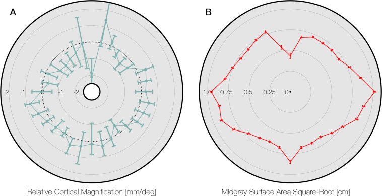
Appendix 1—figure 3. Comparison to Silva et al., 2018.

(A) Data from Silva et al., 2018; Figure 4, replotted around the visual field. The gray area of the panel indicates the axis limits of the original plot. Plot points and confidence intervals represent the linear cortical magnification of each polar angle bin after regressing out the effect of eccentricity on cortical magnification. (B) The square root of the mid-gray surface area of the 163 subjects analyzed in this paper, plotted for polar angle bins matched to those in panel A. Bins were limited to between 1° and 6° of eccentricity. The square-root of the surface area is used because it should scale linearly with the linear cortical magnification values plotted by Silva et al., 2018 and replotted in panel A. Notably, the LVM has a substantially higher surface area in panel B than the points around it. This is likely due to the prevalence of ipsilateral pRFs near the LVM (Gibaldi et al., 2021). Our method does not explicitly account for ipsilateral representation, and thus parts of cortex with ipsilateral pRFs will tend to be counted as part of the vertical meridian when the polar angle bins are sufficiently small (see also Methods). Thus the data point at the LVM should be read and interpreted with caution. pRF, population receptive field. LVM, lower vertical meridian.