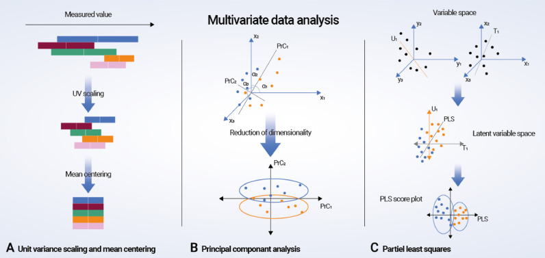
Fig. 3.
Multivariate data analysis. (A) Preprocessing of metabonomic data using unit variance scaling and mean centering. (B) Principal component analysis (PCA, D2): a virtual matrix X is created with a number of observations (n spectra) and K variables (metabolites). A variable space is constructed with as many dimensions as variables; each variable is characterized by one coordinate axis, but for illustrative purposes, only three variable/metabolite axes (x1, x2, and x3) are displayed. Each observation from the matrix X is then placed in the K-dimensional variable space and mean centered around the value zero, creating a cloud of data points. PCA in this space results in lines or principal components (PrCs) that approximate the variables as closely as possible by reducing correlated variables to a smaller set of uncorrelated variables (PrCs). If the first two PrCs account for 80% of the total variation, only 20% of the total variation will be lost by this two-dimensional reduction. The observation points are projected onto the two-dimensional plane, resulting in new coordinate values for each observation (known as scores), and this makes it possible to produce a PrC score plot. Understanding the scores is possible by calculating loadings, which are given by cosines of the angles α1, α2, and α3 to each PrC. Loading values define the way in which the original variables are linearly combined to form the new variables or PrCs and unravel the degree of correlation and in what manner (positive or negative correlation) the original variables contribute to the scores. (C) Partial least squares (PLS) regression: mean-centered and scaled fabricated x and y data sets are demonstrated as a cloud of points in each variable space. Only three variable axes are displayed, respectively (x1, x2, x3 and y1, y2, y3). PLS regression analysis results in linear arrangements of the original x and y variables, creating new or “latent” variables (T1 and U2). These latent variables, or x and y scores, are in essence principally identical to PrCs. However, the PLS regression model strengthens the relationship between the x and y axes because the iterative algorithm used exchange scores between the two data sets and consequently defines the latent variables in the x data set that have high covariance with those in the y data set. Covariance is required in each dimension, and once it is identified in one dimension, the x data set is decomposed at the same time as the predicted y data set is created. Thus, PLS regression concurrently projects the x and y variables onto a common subspace (TU) so that there is a close relationship between the position of one observation on the x plane and its corresponding position on the y plane. This creates a PLS regression component for the first modeled dimension T1 and U1. The second PLS regression component is created in a similar fashion, and the subsequent PLS data can be illustrated as score and loading plots.

