Fig. 14.

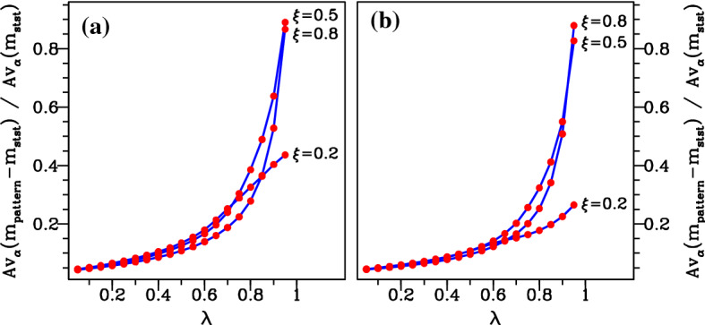
Quantitative details of the comparison between the average mussel density in spatial patterns and the steady-state mussel density. In (a, b) the migration speed and wavelength, respectively, are held constant at their value at pattern onset (the Turing–Hopf bifurcation point); examples of the two corresponding solution branches are shown in Fig. 9. For each pair of $\lambda$ and $\xi$ values, we used the software package wavetrain (Sherratt 2012) to track the form of the pattern along these solution branches as $\alpha$ is varied with the other parameters fixed. We then calculated the average over $\alpha$ of the difference between the mean mussel density and the steady-state mussel density and divided this by the average of the steady-state mussel density. This gives a single number comparing the mussel density in spatial patterns and in the steady state, and we plot this as a function of $\lambda$ for $\xi =0.2$, 0.5 and 0.8. The plots show an increasing separation between the pattern and steady-state solution branches as $\lambda$ is increased between 0 (increased production model) and 1 (decreased losses model). However, there is no clear trend in the way in which the difference in mussel densities varies with the parameter $\xi$. The other parameters are $\beta =0.1$ and $\nu =100$