Fig. 5.

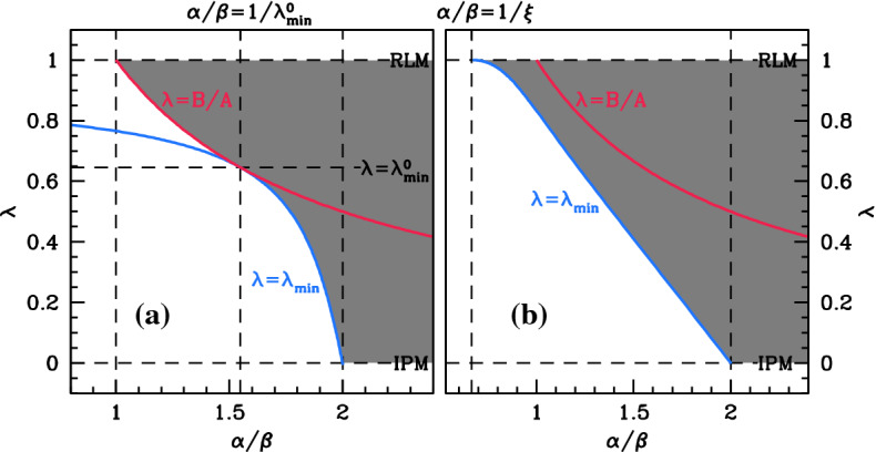
Existence of a positive stable steady state. The shading shows typical examples of the parameter region for which model () has a positive steady state that is stable to homogeneous perturbations, for a $\xi <1$ and b $\xi >1$. The blue curve is the locus of ${\lambda }_{\text{min}}$, calculated by a two-parameter numerical continuation using auto (Doedel 1981; Doedel et al. 1991, 2006), with $\lambda$ and $\alpha$ as continuation parameters. The red curve is $\alpha /\beta =1/\lambda$: the mussel-free steady state $a=\alpha$, $m=0$ is stable below this curve and unstable above it. The parameter values used for the plots were $\beta =0.1$ and a $\xi =0.15$, b $\xi =1.5$