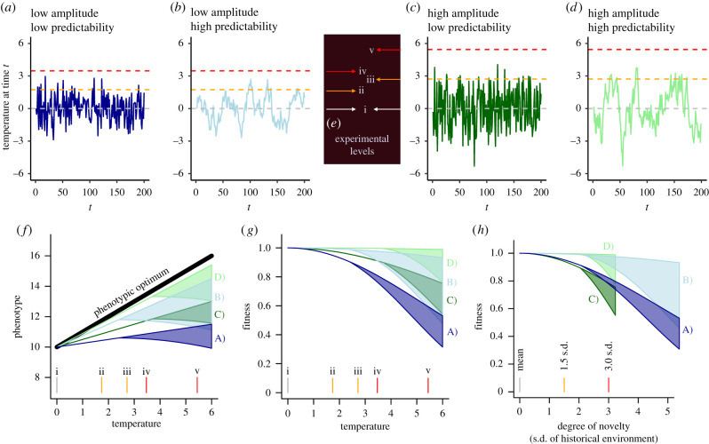
Box 2 figure 1.

(a–d) Examples of time series with different amplitudes and predictabilities. The horizontal orange and red lines represent 1.5 and 3.0 standard deviations (σ) of the historical environment, respectively (e.g. degree of novelty). The timescale could be small (e.g. hours or days) or large (e.g. years), but should be relevant to the timescale between development of the phenotype and selection (see box 1). (e) Experimental levels for the assessment of reaction norms and fitness under future environments, which would allow for both absolute and relative degree of novelty comparisons. (f–d) Theoretical expectations for evolved reaction norms and patterns of fitness across temperature conditions that are informed by the time series data and experimental levels depicted in (a–d). (f) Hypothetical examples of reaction norms that evolve in each of the four time series in A–D, following the theoretical prediction that predictability is the primary determinant of reaction norm slope. The transparent shaded areas represent uncertainty in the value that the phenotype would have in novel conditions (greater than 2σ of the historical temperature). The black line shows the phenotypic optimum for different values of the environment. (g) Fitness based on stabilizing selection acting on each phenotype, assuming no cost to plasticity. (h) The same plot as (g), but the x-axis was rescaled to represent the degree of novelty (σ) of the historical environment, showing how populations that evolved in environments with similar predictability may have similar fitness as a function of novelty. Source code for the generation of this figure is provided in electronic supplementary material, file S1.