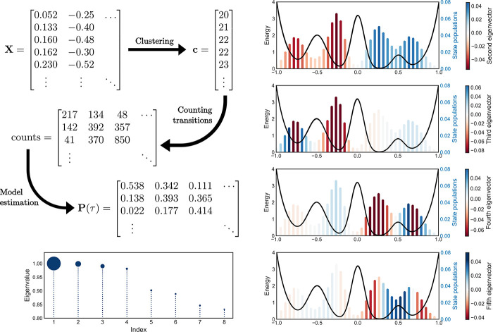
Figure 7.

Schematic illustration describing the MSM construction. First, the data X is reduced to a sequence of integer states c. Then, transitions among those states after a duration of a lag time τ are counted and stored in a count matrix. Next, the MSM itself is estimated from the count matrix to create a transition matrix P(τ). The eigenvalues of P(τ) correspond to the time scales of the process according to t_α ≡ −τ/log|λ̂_α|. The sizes of circles in the bottom left plot correspond to time scale magnitudes; it can be observed that small changes in eigenvalues result in large changes in time scales due to the logarithmic transformation. On the right, the state populations are shown for the first four dynamical eigenvectors (corresponding to eigenvalue indexes 2–5), along with the underlying potential. The heights of the bars indicate state populations, and the colors indicate flux into (blue) and out of (red) various states.