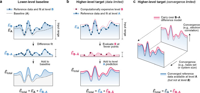
Figure 18.

Overview of different approaches to the hierarchical fitting of potential-energy surface (PES) models. In this figure, the actual PES are labeled E; fitted models are labeled ; the indices A and B refer to different types of PES. Drawings are based on the presentation in ref (164). (a) Using a lower-level baseline model, which might be a simple analytical term that only describes certain aspects of the PES (e.g., pair repulsion, fixed-charge electrostatics, or London dispersion) or a fast semiempirical method. The baseline model is subtracted from the reference data before the fit, resulting in a difference model, _B–A, to which the baseline model E_A is then added back when predictions are made. (b) Fitting a higher-level target: for a suitably chosen baseline, the difference fitting target is smoother (e.g., the range of input data is smaller, or the difference target varies on a larger length scale), and therefore fewer reference points are required. Here, in the subscript of indicates that the fit was made to a potential-energy difference where the fitting target was obtained by subtracting a fitted model of PES A from the actual PES B. (c) A more complex setup in which convergence (e.g., with basis set or system size) can be achieved for level A but not for B, which might be because B uses a higher level of treatment for electron correlation and therefore is more computationally costly.