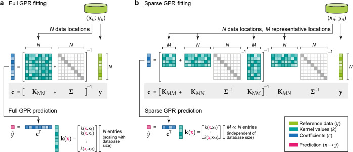
Figure 4.

Visualization of the matrix equations that define the fitting of full (eq 14) and sparse (eq 11) GPR models, and the way they are used for prediction. (a) The reference database consists of entries {x_n; y_n}; the data labels y₁ to y_n are collected in the vector y (light green); the data locations x₁ to x_N are used to construct the kernel matrix, K, of size N × N (teal). The regularizer, Σ, is shown as a light gray diagonal matrix. By solving the linear problem, the coefficient vector c (blue) is computed, and this can be used to make a prediction at a new location, (x) (eq 12), the cost of which scales with the number of data locations, N. (b) In sparse GPR, the full data vector y is used as well, but now M representative (“sparse”) locations are chosen, with M ≪ N. The coefficient vector is therefore of length M, and the cost of prediction is now independent of N.