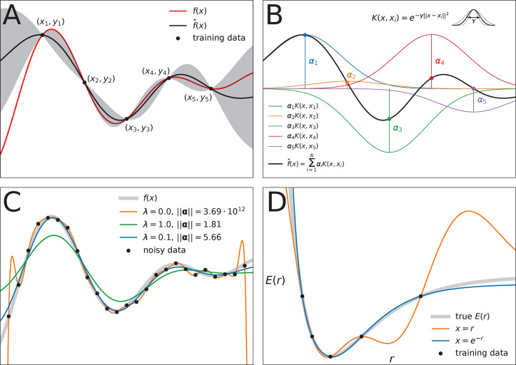
Figure 6.

Overview of the mathematical concepts that form the basis of kernel methods. (A) Gaussian process regression of a one-dimensional function f(x) (red line) from M = 5 data samples (x_i, y_i). The black line (x) depicts the mean (eq 8) of the conditional probability p(|y) (see eq 7), whereas the gray area depicts two standard deviations from its mean (see eq 9). Note that predictions are most confident in regions where training data is present. (B) Function (x) can be expressed as a linear combination of M kernel functions K(x, x_i) weighted with regression coefficients α_i (see eq 2). In this example, the Gaussian kernel (eq 4) is used (the hyperparameter γ controls its width). (C) Influence of noise on prediction performance. Here, the function f(x) (thick gray line) is learned from M = 25 samples, however, each data point (x_i, y_i) contains observational noise (see eq 6). When the coefficients α_i are determined without regularization, i.e., no noise is assumed to be present, the model function reproduces the training samples faithfully, but undulates wildly between data points (orange line, λ = 0). The regularized solution (blue line, λ = 0.1, see eq 10) is much smoother and stays closer to the true function f(x), but individual data points are not reproduced exactly. When the regularization is too strong (green line, λ = 1.0), the model function becomes unable to fit the data. Note how regularization shrinks the magnitude of the coefficient vectors ∥α∥. (D) For constructing force fields, it is necessary to encode molecular structure with a representation x. The choice of this structural descriptor may strongly influence model performance. Here, the potential energy E of a diatomic molecule (thick gray line) is learned from M = 5 data points by two kernel machines using different structural representations (both models use a Gaussian kernel). When the interatomic distance r is used as descriptor (orange line, x = r), the predicted potential energy oscillates between data points, leading to spurious minima and qualitatively wrong behavior for large r. A model using the descriptor x = e^–r (blue line) predicts a physically meaningful potential energy curve that is qualitatively correct even when the model extrapolates.