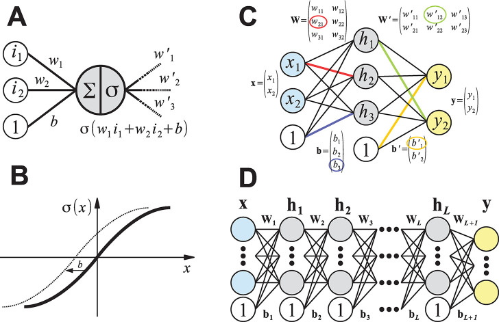
Figure 8.

Schematic representation of the mathematical concepts underlying artificial (feed-forward) neural networks. (A) A single artificial neuron can have an arbitrary number of inputs and outputs. Here, a neuron that is connected to two inputs i₁ and i₂ with “synaptic weights” w₁ and w₂ is depicted. The bias term b can be thought of as the weight of an additional input with a value of 1. Artificial neurons compute the weighted sum of their inputs and pass this value through an activation function σ to other neurons in the neural network (here, the neuron has three outputs with connection weights w′₁, w′₂, and w′₃). (B) Possible activation function σ(x). The bias term b effectively shifts the activation function along the x-axis. Many nonlinear functions are valid choices, but the most popular are sigmoid transformations such as tanh(x) or (smooth) ramp functions, for example, max(0, x) or ln(1 + e^x). (C) Artificial neural network with a single hidden layer of three neurons (gray) that maps two inputs x₁ and x₂ (blue) to two outputs y₁ and y₂ (yellow), see eq 15. For regression tasks, the output neurons typically use no activation function. Computing the weighted sums for the neurons of each layer can be efficiently implemented as a matrix vector product (eq 14). Some entries of the weight matrices (W and W′) and bias vectors (b and b′) are highlighted in color with the corresponding connection in the diagram. (D) Schematic depiction of a deep neural network with L hidden layers (eq 16). Compared to using a single hidden layer with many neurons, it is usually more parameter-efficient to connect multiple hidden layers with fewer neurons sequentially.