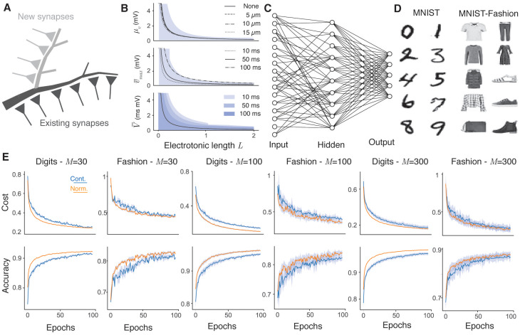
Fig 1. Dendritic normalisation improves learning in sparse artificial neural networks.
A, Schematic of dendritic normalisation. A neuron receives inputs across its dendritic tree (dark grey). In order to receive new inputs, the dendritic tree must expand (light grey), lowering the intrinsic excitability of the cell through increased membrane leak and spatial extent. B, Expected impact of changing local synaptic weight on somatic voltage as a function of dendrite length and hence potential connectivity. Top: Steady state transfer resistance (Eq 10) for somata of radii 0, 5, 10, and 15 μm. Shaded area shows one standard deviation around the mean in the 0 μm case (Eq 11). Middle: Maximum voltage response to synaptic currents with decay timescales 10, 50, and 100 ms (Eqs 14 and 16). Shaded area shows one standard deviation around the mean in the 100 ms case (Eq 15). Bottom: Total voltage response to synaptic currents with the above timescales (all averages lie on the solid line, Eq 17). Shaded areas show one standard deviation around the mean in each case (Eq 18). Intrinsic dendrite properties are radius r = 1 μm, membrane conductivity gl = 5 × 10⁻⁵ S/cm2, axial resistivity ra = 100 Ωcm, and specific capacitance c = 1 μF/cm2 in all cases and Δsyn = 1 mA. C, Schematic of a sparsely-connected artificial neural network. Input units (left) correspond to pixels from the input. Hidden units (centre) receive connections from some, but not necessarily all, input units. Output units (right) produce a classification probability. D, Example 28 × 28 pixel greyscale images from the MNIST [40] (left) and MNIST-Fashion [41] (right) datasets. The MNIST images are handwritten digits from 0 to 9 and the MNIST-Fashion images have ten classes, respectively: T-shirt/top, trousers, pullover, dress, coat, sandal, shirt, sneaker, bag, and ankle boot. E, Learning improvement with dendritic normalisation (orange) compared to the unnormalised case (blue). Top row: Log-likelihood cost on training data. Bottom row: Classification accuracy on test data. From left to right: digits with M = 30 hidden neurons, fashion with M = 30, digits with M = 100, fashion with M = 100, digits with M = 300, fashion with M = 300. Solid lines show the mean over 10 trials and shaded areas the mean ± one standard deviation. SET hyperparameters are ε = 0.2 and ζ = 0.15.

