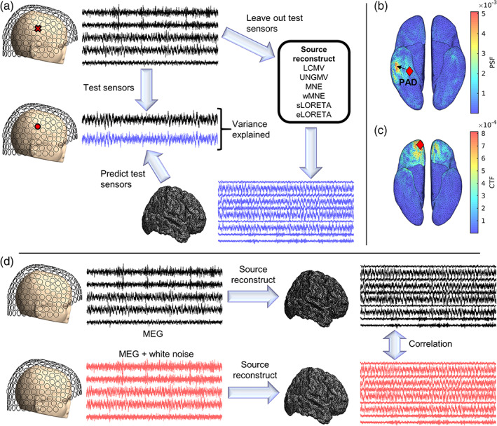
FIGURE 1.

Variance explained analysis methods of comparing source reconstruction algorithms. (a) Variance explained analysis. Two hundred seventy‐four channel MEG data are split into 27 partitions of 10–11 sensors. For each cross‐validation fold, one partition is used as a test data set and all other folds are used as training data. For each algorithm, the training data are source reconstructed to gain an estimate of source dynamics. This source‐reconstructed activity is then forward mapped to the left out test sensors, and the temporal variance of the data recorded at these sensors explained by the brain activity is calculated as squared (temporal) correlation. The $r_{\mathit{CV}}^2$ measure reported here is the average variance explained at each test sensor, averaged over folds. For visualization, we demonstrate a single test sensor. The same methods are repeated for empty‐room recordings, and we use ratio of variance explained in resting‐state versus empty room recordings as our measure of interest. (b,c) Resolution analysis. (b) For a seed voxel, the corresponding column of the resolution matrix (the point spread function; PSF) relates unit “true” activity at that voxel to source estimates at each voxel. The distance between the seed voxel and the voxel at the peak of the PSF is the PAD. Shown is an example PSF for a seed voxel at the red diamond. The arrow points from the seed to the peak of the PSF, and the length of the arrow is PAD. The SEPS is the PSF‐weighted sum of distances to each voxel from the seed. (c) Rows of the resolution matrix (the cross talk function; CTF) quantifies the influence of “true” activity at all voxels on the source estimate of the seed voxel. The SECT is the CTF analogue of SEPS. Here we show an example CTF for a seed voxel at the red diamond. In b,c, figures are plotted on the smoothed cortical surface for visualization purposes only. (d) External noise analysis. To test robustness to external noise, white noise is added to the MEG sensor‐level data. Correlation between source‐space solutions with and without added sensor noise is computed. The level of reduction in correlation as the sensor‐level noise increased quantifies an algorithm's sensitivity to external noise