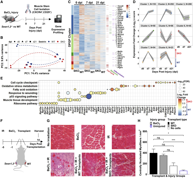
Figure 2.

Sesn1,2 Knockout MuSCs show robust regenerative responses despite having strongly altered basal-level transcriptomes

(A) Schematic diagram of BaCl₂ injury model in the hindlimbs of WT and SKO mice followed by MuSC isolation via FACS and RNA-seq profiling before and during regeneration.

(B) Principal-component analysis (PCA) of MuSC replicates from WT and SKO mice.

(C) Standardized heatmap (Z scores) of 982 differentially expressed genes (SKO over WT) from WT and SKO MuSCs grouped by Dirichlet process Gaussian process (DPGP) clusters. Genes that participate in the cell cycle (Buettner et al., 2015), the Ribosome KEGG pathway (mmu03010), and the muscle cell differentiation gene ontology (GO) term (GO: 0042692) are marked on the right.

(D) DPGP mixture model-based clustering of mean gene expression time series Z scores (gray bars are 2× standard deviation and black line is cluster mean).

(E) Gene set terms and KEGG pathways at 0 dpi plotted against constituent genes.

(F) Schematic diagram for SKO and WT MuSC transplantation experiment. The hindlimbs of young mice (5-month-old males) were irradiated 5 days before transplantation and TAs were injured with an intramuscular BaCl₂ injection or left uninjured 1 day before transplantation. Alternating TAs received either SKO cells (n = 4 mice), WT cells (n = 4 mice), or no cells (n = 3 mice and 4 mice for injured and uninjured controls, respectively) during transplantation. TAs were harvested 2 weeks post-transplantation.

(G) Representative H&E images of TA cross-sections following no injury, only BaCl₂ injury, or only irradiation (top), and following a combination of BaCl₂ and irradiation followed by no cell transplantation, WT cell transplantation, or SKO cell transplantation (bottom). Scale bars, 200 μm.

(H) Quantification of centrally nucleated myofibers per total cross-sectional area (mm²) between transplant groups. Bar plot fill colors indicate transplant type and border colors indicate injury type. Statistical comparisons are two-sided, unpaired Student’s t tests. All data are shown as mean ± SEM. ^∗p < 0.05, ^∗∗∗p < 0.001. See also Figure S3 and Table S1.