FIGURE 4.

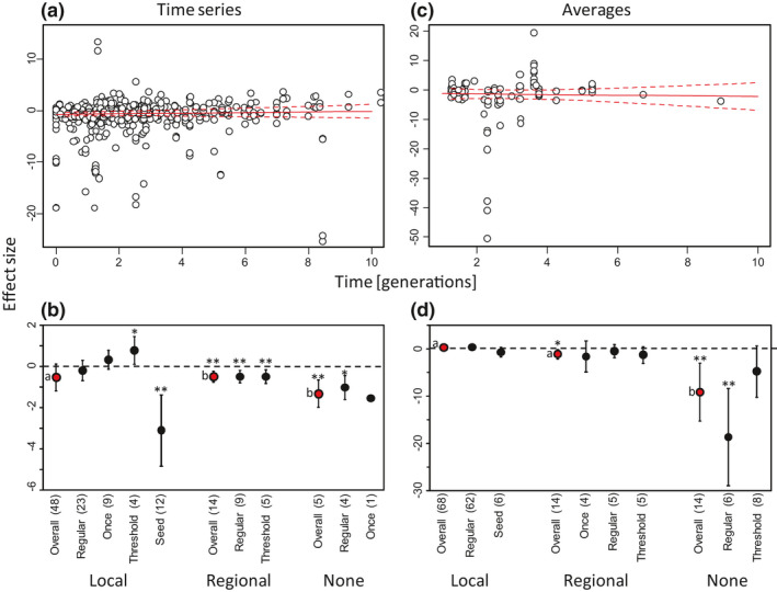
The effect of pesticides on pest densities in field experiments with time series of pest densities (left column) and average pest densities per season (right column). In (a), each point shows the effect size (Hedges g) of one time point of time series of pest densities in time; in (c), each point represents a seasonal average as function of half the length of the total season. Positive values mean a positive effect of pesticides on pest densities. Overall, the trend through time (drawn red line) is close to no effect (zero). (b) and (d) show the effect of the presence of natural enemies and the pesticide application method on pesticide efficacy. (b) shows effects on repeated measures of studies reporting time series; (d) shows effects of studies presenting long‐term average pest densities. Local: natural enemies were present locally; Regional: natural enemies were reported from the same region but not in the publication evaluated; None: no record of natural enemies. Within each of these enemy presence categories, the overall effect (red dots) and the effect per pesticide application method (black dots) are given. Once: pesticides were applied once during the experiment; Regular: pesticides applied several times; Threshold: pesticides were applied according to some damage or pest density threshold; Seed: pesticides were applied to the seeds before planting. Dashed lines in (a) and (c) and error bars in (b) and (d) are 95% confidence intervals. Numbers between brackets after the horizontal axis labels in (b) and (d) give the number of cases, letters next to data points indicate significant differences between overall effects, asterisks indicate significance of the effect: *p < 0.05; **p < 0.01