. 2021 Aug 31;10:e68980. doi: 10.7554/eLife.68980

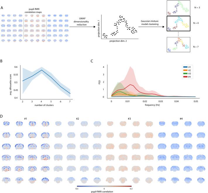
Figure 2. Clustering of trials with distinct pupil–fMRI correlation patterns.

(A) Schematic of the clustering procedure. UMAP is used to reduce the dimensionality of all individual-trial correlation maps to 72 dimensions. A 2D UMAP-projection of the real data is shown. Each dot represents a single trial. The trials are clustered using Gaussian mixture model clustering. Different numbers of clusters are evaluated. (B) The final number of clusters is selected based on silhouette analysis. The highest average silhouette score is obtained with k = 4 clusters. Shaded area shows standard deviations. (C) Pupil power spectral density estimates (PSD) of each of the four clusters. Signals were downsampled to match the fMRI sampling rate. Shaded areas show standard deviations. (D) Cluster-specific correlation maps based on concatenated signals belonging to the respective groups.

Figure 2—source data 1. Cluster trial labels, individual silhouette scores (B), mean cluster PSDs (C), and cluster-specific correlation maps (D) are available in the source data file.

Figure 2.

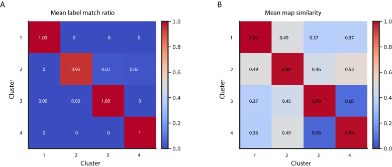
Figure 2—figure supplement 1. Cluster reproducibility across 100 repetitions with random UMAP and GMM initializations.

Figure 2—figure supplement 1.

(A) Matrix displaying the ratio of cluster membership labels matching the most common cluster membership assignment across the 100 repetitions. (B) Matrix displaying the mean spatial correlation between the 100 cluster-specific maps and the maps based on the most common cluster membership assignment.
Figure 2—figure supplement 1—source data 1. The label match ratios (A) and map similarity values (B) are available in the source data file.
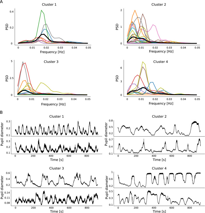
Figure 2—figure supplement 2. Cluster-specific pupil fluctuation features.

Figure 2—figure supplement 2.

(A) PSDs of all trials divided based on their cluster memberships. Clusters 1 and 3 show specific peak frequencies. Cluster 4 shows the largest PSDs, hence the largest pupil size fluctuations. Cluster 1 shows the opposite. (B) Two example pupil diameter time courses are plotted per cluster. The magnitude of changes reflects the PSD differences visible in (A).
Figure 2—figure supplement 2—source data 1. All PSDs (A) are available in the source data file.
All pupil signals (B) are available online (see Materials and methods).
Figure 2—figure supplement 3. Clustering reproducibility across 100 clustering repetitions based on HRF-convolved pupil signals.

Figure 2—figure supplement 3.

(A) HRFs with different peak times were used to create the convolved and lagged pupil signals. (B) Mean match ratio of cluster membership labels created using the convolved signals and those employed throughout the manuscript. The shaded area shows the standard deviation. (C) Mean spatial correlation between cluster-specific maps created using the convolved and non-convolved signals. The shaded area shows the standard deviation.
Figure 2—figure supplement 3—source data 1. The HRF kernels (A), cluster membership label match ratios (B), and map similarity values (C) are available in the source data file.
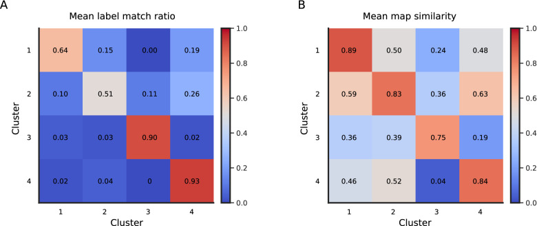
Figure 2—figure supplement 4. Cluster reproducibility across 100 repetitions of split-halves clustering.

Figure 2—figure supplement 4.

(A) Matrix displaying the ratio of split-halves cluster membership labels matching the cluster membership assignment based on all trials across 100 repetitions. (B) Matrix displaying the mean spatial correlation between the 100 split-halves cluster-specific maps and maps based on all trials.
Figure 2—figure supplement 4—source data 1. The label match ratios (A) and map similarity values (B) are available in the source data file.
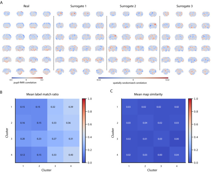
Figure 2—figure supplement 5. Cluster reproducibility across 100 sets of artificially generated surrogates with values and spatial autocorrelations matching those of real maps.

Figure 2—figure supplement 5.

(A) A real pupil–fMRI correlation map and three example surrogate maps. (B) Matrix displaying the ratio of cluster membership labels generated based on the surrogate maps and those based on real data. (C) Matrix displaying the mean spatial correlation between the surrogate cluster-specific maps and those based on real data.
Figure 2—figure supplement 5—source data 1. Ten example surrogate sets (i.e. 740 maps total) (A), label match ratios (B), and map similarity values (C) are available in the source data file.
Figure 2—figure supplement 6. Mean silhouette scores based on 100 clustering repetitions performed on shorter trials.
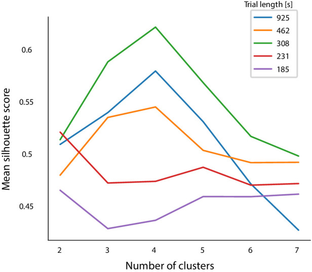
Figure 2—figure supplement 6.

Based on the silhouette score criterion, the n = 4 clusters result should be chosen even when dividing the trials into three parts.
Figure 2—figure supplement 6—source data 1. Individual silhouette scores are available in the source data file.