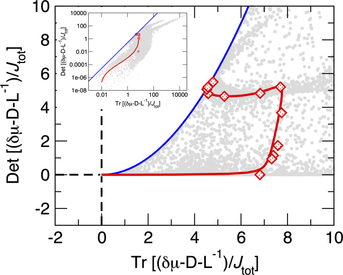
Fig. 4.

Numerical verification of Eq. 10. The blue boundary marks the location of the inequality $\text{Tr}\left[A\right]\ge 2\sqrt{Det\left[A\right]}$ for a two dimensional square matrix $A$. The red diamonds are results from the nonequilibrium KMC simulations with the parameters used in Fig. 2 and the red line is the theoretical mean-field prediction for those same parameters. Gray dots are computed by constructing the matrices $\mathit{\delta }\mathit{\mu }$, $\mathbf{D}$, and ${\mathbf{L}}^{-1}$ using the the master equation results and computing the eigenvalues of $\left(\mathit{\delta }\mathit{\mu }-\mathbf{D}-{\mathbf{L}}^{-\mathbf{1}}\right)/J_{\mathrm{t}\mathrm{o}\mathrm{t}}$ using Mathematica (47) for randomly selected parameters from $L_{\beta ,\mathrm{e}\mathrm{q}}=\left[\mathrm{1,90,000}\right]$, $f_{density,\beta }=\left[\mathrm{1,100}\right]$, and $k_{\mathrm{g}\mathrm{r}\mathrm{o}\mathrm{w}}=\left[0.001,100\right]$ nm/s, with all other parameters the same as the red line. Inset shows these two quantities for a wider range, with both axes on logarithmic scales. We do not consider $k_{\mathrm{g}\mathrm{r}\mathrm{o}\mathrm{w}}<0.001$ nm/s due to limitations of numerical precision. Eq. 1/Eq. 10 provides strong constraints between the nonequilibrium forcing, morphology, and speed of growth.