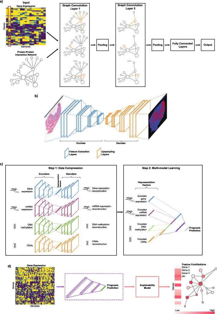
Fig. 2.

An overview of Deep Learning techniques and concepts in oncology. a Graph convolutional neural networks (GCNN) are designed to operate on graph-structured data. In this particular example inspired by [17–19], gene expression values (upper left panel) are represented as graph signals structured by a protein–protein interactions graph (lower left panel) that serve as inputs to GCNN. For a single sample (highlighted with red outline), each node represents one gene with its expression value assigned to the corresponding protein node, and inter-node connections represent known protein–protein interactions. GCNN methods covered in this review require a graph to be undirected. Graph convolution filters are applied on each gene to extract meaningful gene expression patterns from the gene’s neighbourhood (nodes connected by orange edges). Pooling, i.e. combining clusters of nodes, can be applied following graph convolution to obtain a coarser representation of the graph. Output of the final graph convolution/pooling layer would then be passed through fully connected layers producing GCNN’s decision. b Semantic segmentation is applied to image data where it assigns a class label to each pixel within an image. A semantic segmentation model usually consists of an encoder, a decoder and a softmax function. The encoder consists of feature extraction layers to ‘learn’ meaningful and granular features from the input, while the decoder learns features to generate a coloured map of major object classes in the input (through the use of the softmax function). The example shows a H&E tumour section with infiltrating lymphocyte map generated by Saltz et al. [20] DL model c multimodal learning allows multiple datasets representing the same underlying phenotype to be combined to increase predictive power. Multimodal learning usually starts with encoding each input modality into a representation vector of lower dimension, followed by a feature combination step to aggregate these vectors together. d Explainability methods take a trained neural network and mathematically quantify how each input feature influences the model’s prediction. The outputs are usually feature contribution scores, capable of explaining the most salient features that dictate the model’s predictions. In this example, each input gene is assigned a contribution score by the explainability model (colour scale indicates the influence on the model prediction). An example of gene interaction network is shown coloured by contribution scores (links between red dots represent biological connections between genes)