Reconstruction of the incremental capacity trajectories from current-varying profiles for lithium-ion batteries

Summary

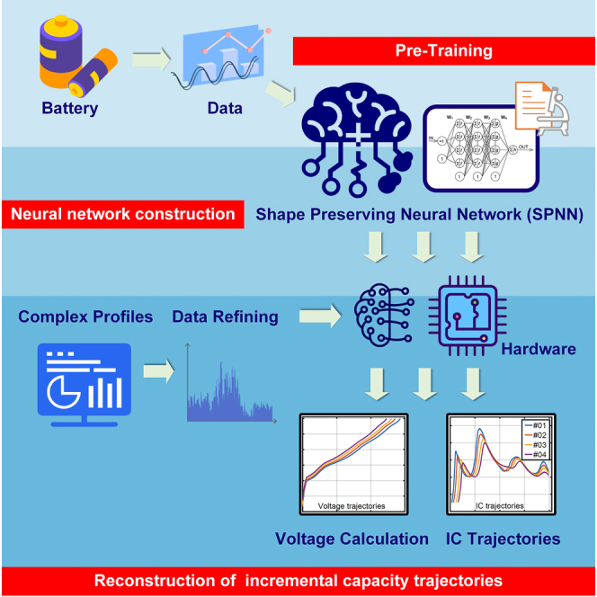
The reliable assessment of battery degradation is fundamental for safe and efficient battery utilization. As an important in situ health diagnostic method, the incremental capacity (IC) analysis relies highly on the low-noise constant-current profiles, which violates the real-life scenarios. Here, a model-free fitting process is reported, for the first time, to reconstruct the IC trajectories from noisy or even current-varying profiles. Based on the results from overall 22 batteries with three case studies, the errors of the peak positions in the reconstructed IC trajectories can be bounded within only 0.25%. With health indicators extracted from the reconstructed IC trajectories, the state of health can be readily determined from simple linear mappings, with estimation error lower than 1% only. By enabling the IC-based methods under complex load profiles, enhanced health assessment could be implemented to improve the reliability of the power systems and further promoting a more sustainable society.

Graphical abstract

Highlights

• •Reconstruct the incremental capacity trajectories from non-constant-current profiles
• •The positioning error of all incremental capacity peaks could be bounded by 0.25%
• •Suitable for single cell/pack with different temperatures, aging, and current rates
• •Developing a shape-preserving transfer learning network for the reconstruction

Electrochemical energy production; Energy storage; Energy materials

Introduction

Literature review

With the advantages of long cycle lifetime, high power and energy densities, lithium-ion batteries are widely used in areas such as the electrified tools, microgrids, electric vehicles, etc (International Energy Agency, 2020; Tian et al., 2021). However, the inevitable battery degradation would result in a decrease in capacity and reduction in power, further influence the performance and reliability of the battery systems (Wang et al., 2021; Lucu et al., 2018). To ensure safe and efficient battery operations, an accurate health diagnostic method is essential for a battery management system (BMS).

The degree of battery aging is commonly represented by the state of health (SoH), which could be defined as the ratio of the battery’s actual capacity to the rated capacity in engineering practice (Tang et al., 2019d). Since the actual capacity cannot be measured in real-life applications due to the incomplete charging-discharging operations (Lu et al., 2013), multiple approaches have been proposed to determine the SoH indirectly from aging-related features. For instance, SoH can be mapped from the electrochemical properties such as the growth of the SEI layer (Crawford et al., 2021) and the increasing of the battery impedance (Cui et al., 2018; Galeotti et al., 2015). However, the in situ extraction of the electrochemical features could be technically challenging and computationally complicated (Zou et al., 2016). In addition, geometry features such as the slope of the charging curves could be easily collected and then mapped to SoH (Yang et al., 2018), but the lack of first-principle explanations reduces the generalizability and reliability of the methods. With the development of data-driven techniques, SoH could also be directly obtained by feeding the raw measurement data into the machine-learning networks (Li et al., 2021), but it could be sophisticated because the health indicators (HIs) have to be extracted from a large amount of raw data with complicated machine-learning tools. When a state-of-charge (SoC) estimator is available, SoH could also be derived by calculating the battery's actual capacity based upon the differential SoC (Jiang et al., 2019). However, the reliable estimation of SoC considering the uncertainties of aging is still an ongoing research topic (Tang et al., 2019b).

In comparison with the aforementioned methods, using incremental capacity analysis (ICA) for health diagnostics has the following advantages (Thompson, 1979). First, since the incremental capacity is defined as the ratio of differential capacity to differential voltage (dQ/dV), its extraction could be much easier than acquiring the electrochemical properties online. Second, the IC trajectories can reflect the electrochemical mechanisms, such as Li-plating (Mei et al., 2020) and intercalation of anions into the graphite-positive electrode (Heidrich et al., 2019). Besides, ICA methods can also be integrated into the data-driven tools (Berecibar et al., 2016), so that the aging-related features could be extracted more efficiently. Lastly, when using ICA methods to determine the SoH, an additional SoC estimator is generally not required. Thanks to these advantages, the ICA-based methods have been widely used in different scenarios such as on-board battery health assessment (Xu et al., 2021), lifetime prediction (Severson et al., 2019), and characterization of the degradation mechanisms (Ouyang et al., 2015).

However, the ICA methods are not perfect. Their implementations rely highly on stable constant current (CC) profiles with low measurement noise (Thompson, 1979), which hinder the popularization of the IC-based battery aging assessments in real-life scenarios. Regarding this issue, multiple research efforts have been reported. In a study by (Li et al., 2018a), Gaussian filtering is proposed to obtain smoothed incremental capacity curves, and then the positions of the extracted IC peaks are applied to estimate the SoH. In a study by (Li et al., 2020), Li et al. decomposed Gaussian-smoothed IC trajectories with a least-squares-based peak fitting algorithm so that the peak values of the IC curves could be protected from being submerged by measurement noise. Torai et al. (Torai et al., 2016) employed the deformed pseudo-Voigt peak function to capture parameters of the IC trajectory, which were further associated with the phase transition of Lithium-ion batteries and used for estimating the SoH. In our previous work (Tang et al., 2018), the “regional capacity” extracted from the IC trajectories is reported to exhibit a relatively stable relationship with SoH under noisy measurements. In Ref (Tang et al., 2020a), rather than considering only one charging-discharging process, multiple operating cycles are considered, and a batch-to-batch Luenberger observer with symmetric moving average filter is developed to extract IC trajectories. In a study by (Maures et al., 2020), the influence of the constant current rates and temperatures on the extraction of IC-based HIs are evaluated, and a logarithmic regression model is developed to achieve accurate SoH estimations.

Motivation and technical challenges

The abovementioned works can well eliminate the influence of different kinds of measurement noises. However, most of these researches are established upon constant current profiles. It is worth noting a “perfect” CC profile is rarely seen in real-life applications. The actual current of the battery might be influenced by multiple effects such as the power supply of the grid (Qin et al., 2021), the current-controlling precision of the charger (Shabshab and Opila, 2016), the employment of the additional battery equalization (Tang et al., 2020c), and even the specifically designed pulse charging profiles (Li et al., 2019; Amanor-Boadu et al., 2018). Since the battery's terminal voltage could change immediately with the current due to the ohmic effects (Tang et al., 2019c), the dynamics of the load profile, rather than the battery's electrochemical behaviors, would dominate the values of the 1/dV term for a current-varying profile. In this case, the information of battery degradation would be merged by the changing load, significantly influencing the performance of ICA methods and hinders the popularization of the IC-based methods in industrial applications. Given the broad applications of the ICA methods such as facilitating SoH estimation (Tian et al., 2019; Feng et al., 2018), classifying battery aging mechanisms (Wang et al., 2018), determining the electrical conductivity (Yi et al., 2020), and assisting the battery lifetime predictions (Severson et al., 2019), a new approach that can extend the ICA methods for complicated load profiles is worthwhile discussing.

Objective and technical contributions

The objective of this work is to reconstruct the IC trajectories from complex load profiles including those with large noises or non-constant-current profiles. In this way, the IC-based method could be extended from laboratory experiments to more real-life applications where the load profiles are highly dynamic.

We here make the first attempt to reconstruct the incremental capacity trajectory from complex load profiles. The reconstruction problem is initially formulated as a curve-fitting problem, and an easy-to-implement averaging-based method is proposed to select the representative data from the complex load profiles. A shape-preserving method is then developed in this paper to fit the selected data and generate smoothed IC trajectories. Three case studies, including the conditions of large measurement noise, pulse charging, and pack charging with the active equalization, are carried out to verify the proposed method. From the experimental results of overall 22 batteries with different aging degrees (obtained from the cyclic aging tests in our previous work (Tang et al., 2019a)), the proposed method can accurately capture the positions of the peaks in the IC trajectories, with an error bounded by 0.25% only. Although the SoH estimation is not considered as the main target of this paper, it can still be accurately determined with an error bounded by 1%. Since the proposed method does not rely on a specific battery model, it can be directly applied to different battery types, paving the way to effective and reliable battery health assessment.

Results

In this section, the proposed method (see STAR Methods) is experimentally verified upon three different using scenarios, namely (1) CC charging with large measurement noise for single batteries, (2) pulse charging for single batteries, and (3) CC charging for battery pack considering the active battery equalization. In addition, the SoH of the battery pack is also estimated based upon the reconstructed IC trajectories.

Case 1: Constant current charging with measurement noise

Background

Different to the cases in the laboratory where low-noise experimental platforms are commonly available, the measurements in general industrial applications are commonly noise polluted (Wei et al., 2020). In the field of battery monitoring, the voltage measurement noise of some latest devices can be well-controlled (e.g., LTC6810, ≈USD 1.1 per channel, maximum error: ±1.8mV), but the measurement error will increase significantly when low-cost platforms (e.g., BQ76925, ≈USD 0.11 per channel, maximum error ±8mV) are applied, posing significant challenges to the implementation of the IC-based in situ battery health diagnostics. In this concern, the noise-canceling performance of the IC extraction algorithm should be verified.

Configurations

In this section, four SONYUS18650VTC5 batteries (rated capacity: Q_nom = 2.5Ah) with different degree of aging are selected, where the newest cell (#01) is utilized for establishing the activation function g(⋅) and initializing of the neural network shown in Figure S5, while the other three batteries are utilized for verification. The SoH of these four batteries (the SoH here is defined by SoH = Q/Q_nom, where Q is the actual capacity) are listed in Table 1, and their voltage trajectories together with the referenced IC values are shown in Figure 1. Here, the experimental data is collected by a 5V30A Ykytech battery testing system, whose maximum measurement error is ±0.05% under full temperature range, and a typical error of 0.02% could be achieved under room temperature.

Table 1.

SoH of the selected batteries for single-cell testings (in %)

Cell no.	#01	#02	#03	#04
SoH	96	93.6	88.4	87.2

Figure 1.

Performance of the selected batteries.

(A) Voltage vs time trajectories.

(B) IC vs voltage trajectories.

In this case study, measurement noises with root-mean-squared-error (RMSE) 4mA and 4mV are added to current and voltage measurement, respectively. As an illustration, the histogram of the voltage measurement noise is shown in Figure 2. It is straightforward to see that the maximum value of noise already exceeds 10mV (the frequency is 1.35%), which agrees with the typical situation of the low-cost battery monitoring platforms. When extracting the ICA, the charging rate is selected as 0.2C following the typical results released by the Service and Management Center for electric vehicles (SMC-EVs) (Hong et al., 2019).

Figure 2.

Distribution of the voltage measurement noise.

Results

The voltage, current, and IC trajectories of cells #02, #03, and #04 are shown in Figure 3. The errors of the peak values and peak positions are also listed in Table 2.

Figure 3.

IC reconstruction results for CC charging with measurement noise.

(A): Voltage and current trajectories of Cell #02.

(B) Voltage and current trajectories of Cell #03.

(C) Voltage and current trajectories of Cell #04.

(D) IC trajectories of Cell #02.

(E) IC trajectories of Cell #03.

(F) IC trajectories of Cell #04.

Table 2.

Errors of the values and positions of the IC peak (in %): Case 1

Peak no.	1	2	3	4
Cell #02
Value	0.002	−0.569	0.134	−0.155
Position	−0.031	0.016	−0.125	−0.006
Cell #03
Value	−0.776	0.03	0.558	0.123
Position	0.001	0.019	0.056	0.012
Cell #04
Value	0.338	−0.189	0.9	−0.096
Position	−0.033	−0.038	0.028	−0.029

From these results, it can be seen that the proposed method can accurately recover the IC trajectories from noisy measurements. The errors of the peak values can be well controlled within 1%, while that of the peak positions can be bounded by 0.2% for batteries with different aging degrees. Such a high accuracy verifies that the proposed algorithm is effective for constant-current charging profiles with large measurement noises.

Case 2: Pulse charging

Background

Compared with the commonly used constant-current-constant-voltage charging, a pulse charging strategy has been reported to be helpful in eliminating concentration polarization, increasing the power transfer rate, and lowering charge time (Li et al., 2001; Mayers et al., 2012). Proper design of pulse charging can improve the efficiency of the charging processes (Amanor-Boadu et al., 2018), the discharging capacity of the cell (Li et al., 2019), and slightly decrease the rate of battery degradation (Kannan and Weatherspoon, 2020). However, the additional current pulses make the charging process no longer a CC process. In such a case, the determination of the IC trajectory becomes more challenging. To our best knowledge, a solution for IC trajectory extraction under pulse charging conditions has not been reported.

Configurations

Similar to case 1, the same four SONY batteries are selected, where the newest cell (#01) is utilized for modeling, and the three other batteries are utilized for verification. To be specific, the proposed method is verified under 0, 25 and 45^∘C. A cyclic pulse charging profiles are implemented with our abovementioned Ykytech testing platform. For 0 and 25^∘C, the cyclic profile contains a 300-s CC charging with 0.5A (0.2C), followed by a 10-s idling, and a 10-s CC discharging with −1.0A. For the 45^∘C-case, the amplitude of the 300-s CC charging becomes 0.625A (0.25C) to test the algorithm's adaptability to different current rates. With the introduction of zero current and negative current, the new profile becomes highly dynamic.

Results

The voltage responses of the pulse charging together with the reconstructed IC trajectories of cells #02, #03, and #04 under 25^∘C are shown in Figure 4, whereas the results of 0 and 45^∘C could be found in Figures S1 and S2 of the supplemental information. The errors of the peak values and peak positions are listed in Table 3.

Figure 4.

IC reconstruction results for pulse charging under 25^∘C.

(A) Voltage trajectories of Cell #02

(B) Voltage trajectories of Cell #03.

(C) Voltage trajectories of Cell #04.

(D) IC trajectories of Cell #02.

(E) IC trajectories of Cell #03.

(F) IC trajectories of Cell #04.

Table 3.

Errors of the values and positions of the IC peak (in %): Case 2

Profiles	0°C, 0.2C pulse charging				25°C, 0.2C pulse charging				45°C, 0.25C pulse charging
Peak no.	1	2	3	4	1	2	3	4	1	2	3	4
Cell #02
Value	−6.879	−2.609	−1.714	NAa	−5.031	−0.85	−0.172	−1.65	−1.604	−0.825	−0.47	−0.969
Position	0.087	0.019	−0.033	NAa	0.034	0.049	0.052	0.04	0.054	−0.028	−0.114	0.022
Cell #03
Value	−4.361	−3.128	−2.13	NAa	−3.902	−2.143	−0.561	−1.534	−1.356	−0.738	−0.037	−1.347
Position	0.11	0.006	−0.239	NAa	0.06	0.092	0.083	0.05	0.042	0.018	−0.009	−0.013
Cell #04
Value	−3.876	−1.591	0.181	NAa	−3.119	−2.021	−0.087	−0.15	−1.027	−0.125	0.726	−0.894
Position	0.079	0.125	−0.179	NAa	0.032	−0.01	−0.056	0.085	0.017	0.028	−0.108	−0.032

^aThe IC peak has not been fully observed when the cut-off condition of the battery is reached.

As shown in Figure 4B, thanks to the introduction of the negative pulse discharge during the charging process, the selected “time vs voltage” points (yellow) from Algorithm 2 are lower than the referenced values. In addition, some disturbances caused by the polarization effect (Song et al., 2017) can also be observed. These effects could inevitably influence the precision of the extracted trajectories. However, it is interesting to see that the reconstructed IC trajectories are smooth, even though the selected “input-output” data points are still noise-polluted. The primary reason is that the network for fitting the “voltage vs time” relationship does not contain discontinuous activation functions such as “poslin (⋅)”, and it has been pre-trained to a state close to the local optimum. Even though the smoothness of the collected data is highly influenced by the pulses introduced to the charging processes, the peak positions of all batteries can be accurately determined, with an error bounded by 0.25%. Importantly, the proposed method could be directly extended to a wider temperature range (0∼45^∘C) and is tolerable to the small change of the current rate. This result implies that the reconstructed IC trajectories can be used for many applications such as battery health assessment (Tang et al., 2018) or determination of the degradation mechanisms (Ouyang et al., 2015).

Algorithm 2. Collecting the inputs and outputs.

1: n = 0//Index initialization

2: ${\hat{I}}_{1:H}^{\text{SM}}=$MovAvg(I_1:H,M)//Current smoothing

3: ${\hat{V}}_{1:H}^{\text{SM}}=$MovAvg(V_1:H,M)//Voltage smoothing

4: for j = 1,2,⋯,H do

5:  if $|{\hat{I}}_j^{\text{SM}}-I^{\text{∗}}|<\epsilon$ then//Intersection detected

6:  n←n+1//Update the index

7:  $V_n^R={\hat{V}}_j^{\text{SM}}$ //Voltage recording

8:  $t_n^R=j\cdot {\sum }_{k=0}^j\left(I_k\right)/{\sum }_{k=0}^j\left(I^{\text{∗}}\right)$ //Time updating

9:  end if

10: end for

11: return $t_{1:n}^R$, $V_{1:n}^R$

Case 3: Pack charging considering the active balancing

Background

In general industrial applications, hundreds or even thousands of batteries are usually interconnected in series and parallel to satisfy the specific power requirements. However, the inter-cell inconsistency is becoming an inevitable problem that increases with the increment of the number of cells in the battery pack (Turksoy et al., 2020). Batteries with lower actual capacity will, in general, be the first ones to reach and dominate the cut-off conditions of the entire pack. On the one hand, the early cut-off of the charging/discharging processes could waste the underutilized energy stored in other batteries. The degradation of the weakest battery will be accelerated (Tang et al., 2020b) if it always suffers from deep-charge/discharge, resulting in positive feedbacks and accelerated degradation rate of the entire pack.

Aiming at these issues, the battery balancing (equalization) platforms that can transfer energy among cells are commonly carried out in large-scale battery pack applications (Wu et al., 2019). As additional charging/discharging among cells are inevitable during the equalization process, the actual currents of the batteries in the pack would become non-constant, and the corresponding terminal voltage will also be influenced by the changing current, leaving technical challenges to the extraction of the IC trajectory. Noting that the overall battery capacity in large-scale pack applications such as EVs exceeds 70GWh (International Energy Agency, 2020), the employment of active balancing becomes a bottleneck for the popularization of IC-based in situ battery diagnostics. Similar to the case of pulse charging, an effective approach for IC trajectory extraction considering the active balancing effect has not been reported in the community.

Configurations

In addition to the four batteries used in the first two case studies, another 18 batteries of the same type are connected in a 6-series-3-parallel configuration. Following the common engineering practice, each parallel group is treated as a “big battery”, with a nominal capacity of 7.5Ah. The SoH of these 18 batteries are given, respectively, in Table 4. For pack applications, the operations are implemented with a 100V20A Estar battery pack testing platform and a customized BMS. The photo of our platform is shown in Figure S7, and the operating principle of the hardware is given in Figure S8. Full specifications of our experimental platform can be found in STAR Methods, with the detailed balancing algorithms provided in Algorithms 6 and 7. It is worth noting that for the purpose of generating referenced IC trajectories reliably, the balancing currents of each parallel group are measured in this work. However, when implementing the proposed algorithm, we followed the engineering practice and used the nominal balancing current for calculations. According to Figure S8, the sampling/control is implemented at a frequency of 1Hz, and in each operating cycle, the balancing hardware works for 950ms, leaving 50ms for sampling, calculating, and necessary communications.

Table 4.

SoH of the selected batteries for battery pack testings (in %)

Group no.	G01			G02			G03			G04			G05			G06
Cell no.	#05	#06	#07	#08	#09	#10	#11	#12	#13	#14	#15	#16	#17	#18	#19	#20	#21	#22
SoH	84.4	86.8	90	90.4	94	90	95.6	87.6	92	99.6	99.6	98.8	98.4	98.4	98.4	95.2	95.6	97.6

Algorithm 6. VoltageBal(V).

1: for k = 1,2,⋯ do

2:  E_V(k) = V(k)−mean(V(k))//Tracking References

3:  $\delta V\left(k\right)=\text{max}\left\{{\mathit{E}}_V\left(k\right)\right\}-\text{min}\left\{{\mathit{E}}_V\left(k\right)\right\}$

4:  if $\delta V\left(k\right)\ge 5$mV then//Threshold 01

5:  Discharge the cell with the HIGHEST voltage

6:  PackState = 01

7:  else if $\delta V\left(k\right)\le 2.5$mV then//Threshold 02

8:  Stop the balancing hardware

9:  PackState = 02

10:  else

11:  if PackState = = 01 then

12:  Discharge the cell with the HIGHEST voltage

13:  else

14:  Stop the balancing hardware

15:  end if

16:  end if

17: end for

Algorithm 7. BCRBal(BCR).

1: for k = 1,2,⋯ do

2:  ${\mathit{E}}_B\left(k\right)=\mathbf{B}\mathbf{C}\mathbf{R}\left(k\right)-\mathbf{B}\mathbf{C}{\mathbf{R}}^{\text{ref}}$ //Tracking References

3:  $\delta B\left(k\right)=\text{max}\left\{{\mathit{E}}_B\left(k\right)\right\}-\text{min}\left\{{\mathit{E}}_B\left(k\right)\right\}$

4:  if $\delta B\left(k\right)\cdot Q^{\text{pack}}\left(k\right)\ge 80$mAh then //Threshold 01

5:  Discharge the cell with the MAXIMUM E_B(k)

6:  PackState = 01

7:  else if $\delta B\left(k\right)\cdot Q^{\text{pack}}\left(k\right)\le 40$mAh then//Threshold 02

8:  Stop the balancing hardware

9:  PackState = 02

10:  else

11:  if PackState = = 01 then

12:  Discharge the cell with the MAXIMUM E_B(k)

13:  else

14:  Stop the balancing hardware

15:  end if

16:  end if

17: end for

In this section, the constant charging current is selected to be 0.2C (1.5A) following Ref (Hong et al., 2019), and a balancing-current-ratio-based balancing scheme (Tang et al., 2020c) (see also the STAR Methods) is applied to implement the pack balancing. The data utilized for algorithm verification are collected by our embedded BMS, rather than the Estar testing platform, to simulate real-life using scenarios that contain both varying current and measurement noises. The referenced voltage and IC trajectories are collected by using the above-mentioned Ykytech platform to test each 7.5Ah parallel-connected group. Again, the identification of the g(⋅) function and the network initialization are implemented based upon cell #01.

Results

The current trajectories of the six battery groups are shown in Figure 5, the reconstructed IC trajectories are shown in Figure 6, with errors given in Table 5.

Figure 5.

Actual charging current of the six battery groups.

(A): Group G01.

(B): Group G02.

(C): Group G03.

(D): Group G04.

(E): Group G05.

(F): Group G06.

Here, the actual charging current is obtained by adding the pack current with the balancing current. The desired charging current is 0.2C (1.5A), while the balancing current is jointly determined by the states of the batteries and the balancing scheme. Details of the balancing scheme could be found at STAR Methods. In general, cells with lower capacities are more frequently discharged by the balancing hardware in a charging process to prevent them from reaching the cut-off condition too early.

Figure 6.

IC reconstruction results of the pack applications.

(A): Group G01.

(B): Group G02.

(C): Group G03.

(D): Group G04.

(E): Group G05.

(F): Group G06.

Table 5.

Errors of the values and positions of the IC peak (in %): Case 3

Peak no.	1	2	3	4
G01
Value	−1.184	0.213	−0.243	0.729
Position	0.002	−0.008	−0.004	0.008
G02
Value	−1.448	0.372	0.586	−0.002
Position	−0.02	−0.042	−0.039	−0.164
G03
Value	−0.877	1.169	0.238	−0.100
Position	−0.019	0.006	−0.059	−0.077
G04
Value	−0.589	1.241	0.394	NAa
Position	−0.014	−0.013	−0.079	NAa
G05
Value	−0.768	1.186	0.689	NAa
Position	−0.014	−0.008	−0.077	NAa
G06
Value	−2.024	0.584	0.346	1.062
Position	−0.012	0.084	−0.151	−0.220

^aThe IC peak has not been fully observed when the cut-off condition of the pack is reached.

It can be seen from Figure 5 that the current trajectories are highly chattering, primarily due to the frequent operations of the switch array as shown in Figure S7C. However, the ohmic voltage changes caused by the time-varying current are not covered since the voltages are measured at the end of each operating cycle where the balancing hardware is not working (see Figure S8). As a result, the chattering issue of the raw IC trajectories in this test is less significant than that of case study 2. However, the IC trajectory extraction here is still non-trivial because we can only use typical values of the balancing current for calculation. The inaccurate current measurement also introduces errors to the reconstructed IC trajectories. As revealed in Table 5, with the existence of inaccurate current measurements, the accuracy of the peak values may exceed 1% in some cases. However, the precision of the peak positions can still be controlled within 0.25%, illustrating the effectiveness of the proposed method. To the best of our knowledge, this is the first report of extracting the IC trajectories from a battery pack considering the active balancing issue.

Case 4: state-of-health estimation

Background

Under the framework of IC-based SoH estimation, the overall procedure can be categorized into two sub-steps: (1) Extract the IC trajectories from the complicated load profiles; and (2) Use the extracted IC trajectories to estimate the SoH. Although step 1 is the main focus of this work, it is still important to verify that the extracted IC trajectories could be readily utilized for SoH estimation. For this purpose, a simple SoH estimator is designed in this section. Further information on SoH estimation could be found in our latest reviews (Wang et al., 2020).

Configurations

In this subsection, the batteries #01∼#04 are utilized for modeling, and the SoH of groups G01∼G06 is the target that requires estimating. Given the relatively limited number of training samples, the relationship between the HI and SoH is described by a simple linear function following Ref (Tang et al., 2018, 2021b; Severson et al., 2019)

$$\text{SoH}=k\cdot \text{HI}+b$$ (Equation 1)

where k and b are parameters to be identified. Here, the HI is selected as the charging capacity obtained when the smoothed terminal voltage (from Algorithm 3) raises from the position of the second peak (around 3.7V) to the third peak (around 3.9V) in the charging process following Refs (Tang et al., 2018, 2021b; Severson et al., 2019). Here, we have k = 24.05 and b = 29.11 when setting the unit of HI and SoH as Ah and percentage, respectively (The value of k has been trebled since a parallel-connected group (G01∼G06) contains three batteries).

Algorithm 3. Shape-preserving prediction.

1: function ${\hat{V}}_k$ = SPNNk

2:  IN = k

3:  a_0,b = [IN; 1]

4:  a_1,b = [f(W₁⋅a_0,b); 1]

5:  a_2,b = [f(W₂⋅a_1,b); 1]

6:  a_3,b = [g(W₃⋅a_2,b); 1]

7:  a_4,b = [h(W₄⋅a_3,b); 1]^a

8:  ${\hat{V}}_k=h\left({\mathit{a}}_{4,b}\right)$

9: end function

^aThe values of W_1:4 can be readily trained by a general training algorithm. The training in this paper is implemented by trainlm function in MATLAB, see Data S1 for further details. Another example using gradient correction method can be found in our previous work (Tang et al., 2020b). The network initialization could be implemented by pre-training it using t_1:N and v_1:N, which are originally collected for obtaining (Equation 6).

Results

The SoH estimation results are shown in Figure 7. It can be seen that with the reconstructed IC trajectories, the SoH can be easily estimated from simple linear mappings, with errors bounded by 1% only. Even though the actual battery currents are highly chattering, our accuracy is still competitive to that of the ICA-based SoH estimators with constant current charging profiles (Li et al., 2018a, 2018b, 2020; Chang et al., 2021; Zheng et al., 2018; Weng et al., 2016). These results verify the feasibility of the proposed IC reconstruction method.

Figure 7.

SoH estimation results.

(A) Estimated SoH.

(B) Estimation error.

Discussion

ICA is one of the most important in situ methods for battery health assessment but commonly limited by its reliance on the low-noise constant-current profiles. Aiming at this issue, we reconstruct the IC trajectories from complicated current-varying profiles in this paper. The task is initially formulated as a curve-fitting problem, and an easy-to-implement shape-preserving fitting method is then developed by redesigning the activation functions of the neural network. The IC trajectories are then derived from the well-fitted “voltage vs time” relationship, and the feasibility of our approach is verified based upon battery-in-the-loop experiments on overall 22 batteries with three different using scenarios. Experimental results show that the IC trajectories could be accurately recovered, with peak positioning error bounded by 0.25% for all peaks in all tested cases. Further, with the extracted IC trajectories, the SoH could be accurately estimated, with errors bounded by 1% only, even though it is not explicitly considered as the research target here. This paper is the first report of extracting IC trajectories from complex load profiles such as those considering pulse charging or active pack balancing. Moreover, the proposed method for IC reconstruction is purely model-free, and therefore suitable for general battery types.

Limitations of the study

In this paper, we mainly focus on extracting the IC trajectory from noisy or non-constant-current profiles. However, the detailed utilization of the extracted IC trajectories, such as estimating SoH or determining the battery reaction kinetics with IC trajectories extracted from different temperatures and current rates, are beyond the discussions of this work and require further research efforts. The performance of the proposed method could be significantly reduced if the current rate of interest is so large that the small peaks of in the IC trajectories are submerged. Cost-effective approaches to handle the inaccurate measurements, such as using dual-observer techniques, are also worth discussing. In addition, as a common issue for data-driven algorithms, the lack of physical insights of the battery may reduce the generalization and reliability of the proposed method. This issue could be resolved by introducing the first-principle natures into the data-driven machines, which is an interesting future research direction. It is also interesting to validate the proposed methods for batteries with other chemistries and partial charging profiles in continuation of the work.

STAR★Methods

Key resources table

REAGENT or RESOURCE	SOURCE	IDENTIFIER
Software and algorithms
Related code	This paper	https://doi.org/10.5281/zenodo.5232754
Related data	This paper	https://doi.org/10.5281/zenodo.5232754

Resource availability

Lead contact

All requests for code and data should be directed to the lead contact, A/Prof. Yujie Wang (wangyujie@ustc.edu.cn).

Materials availability statement

This study did not generate new unique reagents.

Method details

Overview

Conventionally, given the time-series response of the battery's terminal voltage with respective to a CC profile, the IC values at time step k could be calculated by

$$I{C}_k=\frac{dQ}{dV}{|}_k\approx \frac{\text{Δ}Q}{\text{Δ}V}{|}_k=\frac{Q_k-Q_{k-L}}{V_k-V_{k-L}}=\frac{{\sum }_{j=k-L+1}^{j=k}\left(I_j\right)}{V_k-V_{k-L}}\cdot \text{Δ}T$$ (Equation 2)

where d is the differentiating operator, Δ is the finite difference operator, Q is the capacity contained in the battery, V is the battery's terminal voltage, I stands for the current, ΔT stands for the sampling interval, and L is the time utilized in the finite-difference.

Since ΔV term is in the denominator, the IC value could be highly sensitive to the fluctuations in the voltage measurement, which may be caused by not only the measurement noise but also the changes in the current (e.g., current-varying profiles). In general, estimating the change in voltage from the given current requires a high-fidelity battery model considering the battery's degradation (Liu et al., 2020). However, one of the most important applications of the IC trajectory itself is to evaluate the aging degree. Therefore, using model-based approaches to estimate the battery's voltage and reconstruct the IC trajectory is infeasible, as this process would lead to circular dependence. In this case, an alternative approach is developed in this paper, where the reconstruction of IC trajectory is formulated as a curve-fitting problem. Noting that the raw IC trajectories are highly chattering under noisy or non-constant-current cases, it could be difficult to determine reliable “IC vs voltage” data pairs to support the curve fitting. Therefore, the aim here is to first reconstruct a “voltage vs time” trajectory of a noise-free constant current profile from the data that may contain non-constant currents and large measurement noises, and then calculate the corresponding IC trajectory following (Equation 2). Under the framework of general curve-fitting, our method can be categorized into three sub-steps:

• 1.Obtain the inputs (time) and outputs (voltage).
• 2.Fit the input-output relationship.
• 3.Calculate the IC trajectories based on the fitting results.

The following discussions starts with the acquiring of the inputs and outputs.

Obtaining the inputs and outputs

The battery's terminal voltage can change with the applied current. Therefore, to obtain the “voltage vs time” trajectory for a specific current rate (denoted by I^∗), only limited data points can be selected from voltage trajectory of a current-varying profiles. To be specific, these selected data points would be extracted from the intersection points between the smoothed current trajectory and a horizontal line y = I^∗, as illustrated in Figure S3A.

Here, the noise-polluted current measurements (denoted as “Actual” in Figure S3) are first smoothed by a standard moving-average filter (Li et al., 2018a), which is detailed in Algorithm 1. To eliminate the influence of the noise, the time-series signals x and y are defined to be intersected at time step k if $|x_k-y_k|<\epsilon$, where ε is a small, positive, real number for noise compensation.

Algorithm 1. Moving average filter.

1: function ${\hat{x}}_{1:H}^{\text{SM}}$ = MovAvgx_1:H, M^a

2:  for j = 1, 2,⋯, H do

3:  if j < M then

4:  ${\hat{x}}_j^{\text{SM}}={\sum }_{l=1}^{l=j}\left(\frac{x_l}{j}\right)$;

5:  else.

6:  ${\hat{x}}_j^{\text{SM}}={\sum }_{l=j-M+1}^{l=j}\left(\frac{x_l}{j}\right)$;

7:  end if

8:  end for

9:  return ${\hat{x}}_{1:H}^{\text{SM}}$

10: end function

^aFor a finite time-series signal x_1:H, the smoothed trajectory ${\hat{x}}_{1:H}^{\text{SM}}$ could be calculated MovAlg(x_1:H, M), where M is the length of the window for moving average, and H is the length of the signal.

Next, the value of the smoothed voltage corresponding to the intersection points are recorded, as illustrated in Figure S3B. With a time-varying current profile, the smoothed voltage response (red curve) exhibits obvious differences to the voltage trajectory of the CC profile where I_j≡I^∗ (purple curve). Therefore, the selected intersection points cannot be directly used for the curve-fitting tasks, even though the voltage points are extracted from the time step when the smoothed current is exactly equal to the target I^∗.

To handle this issue, the input “time” should be re-arranged according to the difference in the current values. To facilitate the descriptions, the time steps corresponding to the intersection points (shown in Figure S3B) are denoted as $[t_1^I,t_2^I,\cdots ,t_n^I]$, where n is the number of the intersection points. Accordingly, the revised time are denoted as $[t_1^R,t_2^R,\cdots ,t_n^R]$. The values of $t_{1:n}^R$ can be calculated by

$$t_j^R=t_j^I\cdot {\sum }_{k=0}^{t_j^I}\left(I_k\right)/{\sum }_{k=0}^{t_j^I}\left(I^{\text{∗}}\right)$$ (Equation 3)

For now, the collection of the input “time” and the output “voltage” has been introduced. As described in Figure S3, these new data points can match the voltage trajectory of the CC profile in a more accurate way and would be used for training the shape-preserving curve-fitting tool described in the next subsection. As a summary, the procedure of collecting these input-output data is given by Algorithm 2.

Shape preserve fitting

In our IC extraction problem, fitting the input-output relationship is non-trivial. The primary challenge comes from the additional requirement of calculating the first-order derivative term (1/ΔV). As illustrated in Figure S4A, most of the commonly used high-order functions (as listed in (Equation 5a), (Equation 5b), (Equation 5c)) can fit the voltage-time relationship accurately, with the root-mean-squared-error (RMSE) (defined in (Equation 4), where z_j stands for the j^th true value of z, ${\hat{z}}_j$ is the j^th estimation of z, and n_z is the total number of estimations considered.) lower than 10mV. However, when calculating the IC trajectories following (Equation 2), the errors become significantly larger, as illustrated in Figure S4B.

$$\text{RMSE}=\sqrt{\stackrel{n_z}{\sum _{j=1}}\frac{{\left({\hat{z}}_j-z_j\right)}^2}{n_z}}$$ (Equation 4)

$$f_{\text{P}9}\left(x\right)=a_0+a_1\cdot x+a_2\cdot x^2+a_3\cdot x^3+\cdots +a_9\cdot x^9$$ (Equation 5a)

$$f_{\text{F}8}\left(x\right)=a_0+a_1\cdot \text{cos}\left(x\cdot \omega \right)+b_1\cdot \text{sin}\left(x\cdot \omega \right)+a_2\cdot \text{cos}\left(2x\cdot \omega \right)+b_2\cdot \text{sin}\left(2x\cdot \omega \right)+\cdots +a_8\cdot \text{cos}\left(8x\cdot \omega \right)+b_8\cdot \text{sin}\left(8x\cdot \omega \right)$$ (Equation 5b)

$$f_{\text{G}8}\left(x\right)=a_1\cdot e^{-{\left(\frac{x-b_1}{c_1}\right)}^2}+a_2\cdot e^{-{\left(\frac{x-b_2}{c_2}\right)}^2}+\cdots +a_8\cdot e^{-{\left(\frac{x-b_8}{c_8}\right)}^2}$$ (Equation 5c)

The primary reason for this effect is that the shape of the first-order derivative trajectory relies highly on the properties of the governing equations. In addition, the nonlinear curve-fitting tools would only minimize the difference between the measured and fitted voltage, without taking the first-order derivative into account. This issue will be exacerbated if the selected input-output data are noise-polluted, increasing the difficulties in developing a mathematical tool that considering the accuracy of both fitting data and the first-order derivative. Provided that only limited data points can be selected for the curve-fitting task, while the selection depends highly on the applied current profiles, determining a reliable approach to avoid over-fitting is also non-trivial.

To sidestep these issues, an alternative data-driven shape-preserving fitting tool is developed. Motivated by the capability of approximating general convex non-linear functions at any desired accuracy (Jones, 1990), the multi-layer-feedforward network (MLFN), as described in Figure S5, is selected to implement the fitting algorithm. However, some modifications should be made to make this network more suitable for the IC-fitting task.

First, g(⋅) in Figure S5 is selected to be the fitted function of “voltage vs time” trajectory as described in Figure S4A. In this way, the new network could contain the prior knowledge of the battery's voltage trajectory over the time. However, as detailed in Figure S4B, selecting a good function for g(⋅) is non-trivial. To guarantee the fitting performance for general battery types, g(⋅) is selected to be non-parametric spline function (Segeth, 2021). To facilitate the following descriptions, we assume N data points can be used to this trajectory, denoted as [(t,v)] = [(t₁,v₁), (t₁,v₂),⋯,(t_N,v_N)]. Then the spline function can be given by

$$g\left(x\right)={\theta }_1\cdot B_1\left(x\right)+{\theta }_2\cdot B_2\left(x\right)+\cdots +{\theta }_N\cdot B_N\left(x\right)$$ (Equation 6)

where θ = [θ₁,θ₂,⋯,θ_N] are the parameters to be identified, and B(x) = [B₁(x),B₂(x),⋯,B_N(x)] are defined by (Hastie et al., 2008)

$$B_1\left(x\right)=1$$ (Equation 7a)

$$B_2\left(x\right)=x$$ (Equation 7b)

$$\begin{array}{cc}{B}_{j+2}\left(x\right)& =\frac{{\left\{\text{max}\left(0,x-t_j\right)\right\}}^3-{\left\{\text{max}\left(0,x-t_N\right)\right\}}^3}{t_N-t_j}\\ & -\frac{{\left\{\text{max}\left(0,x-t_{N-1}\right)\right\}}^3-{\left\{\text{max}\left(0,x-t_N\right)\right\}}^3}{t_N-t_{N-1}}\end{array}$$ (Equation 7c)

To ensure both fitting accuracy and the smoothness of the fitted trajectory, θ in this paper is solved by minimizing the following cost function

$$J\left(\mathit{\theta }\right)=p\cdot \sum _{j=1}^N{\left[v_j-g\left(t_j\right)\right]}^2+\left(1-p\right)\cdot {\int }_{t_1}^{t_N}{\left[\frac{d^{2}g}{d{x}^2}\right]}^{2}dx$$ (Equation 8)

where $p\in \left[\mathrm{0,1}\right]$ is the smoothing parameter, which balances the weight between the fitting error and the smoothness (summation of the second-order derivative) of the fitting. For the task here, p = 10⁻⁶ is selected from trial-and-error method. By defining ${\left\{\mathbf{B}\right\}}_{i,j}=B_j\left(t_i\right)$ and ${\left\{\mathbf{\Omega }\right\}}_{j,k}={\int }_{t_1}^{t_N}{B_j}^{\text{″}}\left(x\right){B_k}^{\text{″}}\left(x\right)dx$, the estimate of θ can be given by (Hastie et al., 2008)

$$\hat{\mathit{\theta }}={\left({\mathbf{B}}^{\text{T}}\cdot \mathbf{B}+\frac{1-p}{p}\mathbf{\Omega }\right)}^{-1}\cdot {\mathbf{B}}^{\text{T}}\cdot \mathit{v}$$ (Equation 9)

Generally speaking, the spline-based fitting method can accurately mimic the relationship between the provided input and output. Therefore, the data utilized for obtaining g(⋅) should be offline measured with high-accuracy platforms to sidestep the influence of the measurement noise. It is worth noting that the battery's voltage curve and, therefore, the IC trajectory could change significantly with temperature and aging. However, once determined as an activation function of a neural network, the g(⋅) is fixed. Aiming at this issue, two conventional layers with the f(⋅) being the activation function are added to the network as described in Figure S5. As proved in (Hartman et al., 1990), a conventional feedforward neural network could approximate any convex nonlinear functions at any desired accuracy provided that sufficient hidden neurons are allowed. By adding more conventional hidden neurons, the information of temperature and aging that submerged in the noisy measurements could be indirectly learned by the network, further improving the overall flexibility of the algorithm.

Though the conventional “s-functions” such as “logsig” or “tansig” are widely used, they suffer from the “data-saturation” issue (Banerjee et al., 2019). In other words, when the range of the input for testing is significantly larger than that for the network training, the output of the “s-functions” will be close to 1 and exhibits negligible changes to the input variations. Therefore, functions with an unbounded output range should be selected. Noting that the first-order derivative of the “voltage vs time” trajectory is important for calculating the IC trajectory, some widely used functions such as Reflected Linear Unit (ReLU) (Banerjee et al., 2019) are not suitable, as they are not smooth at x = 0. In short, the activation function should be continuous, derivable, and exhibit no data saturation effect. Following Ref (Hendrycks and Gimpel, 2016), an enhanced Gaussian error Linear Unit (GeLU) can satisfy these requirements

$$f\left(x\right)=x{\int }_{-\infty }^x\frac{e^{-\frac{t^2}{2}}}{\sqrt{2\pi }}dt$$ (Equation 10)

To simplify the computation, the following approximation is applied

$$f\left(x\right)\approx \frac{1}{2}x\left[1+\text{tanh}\left(\sqrt{\frac{2}{\pi }}\left(x+0.044715x^3\right)\right)\right]$$ (Equation 11)

Finally, the output of g(⋅) are linearly combined to generate the predicted voltage, in other words, h(x) = x is selected. For now, provide an input value of time k, the output voltage V_k can be readily calculated. The detailed procedure is given in Algorithm 3.

Based on Algorithms 1, 2, and 3, the overall procedure of the proposed IC reconstruction procedure can be summarized by Algorithm 4, with the overall block diagram described in Figure S6.

Algorithm 4. Reconstruction of the IC trajectory.

1: Carry out a complete CC charging for a new battery offline

2: Collect the t_1:N and v_1:N data for above process accurately

3: Identify the g(⋅) in (Equation 6) using t_1:N and v_1:N with (Equation 9) offline

4: Collect the raw I_1:H and V_1:H data from the target battery

5: Obtain the training data (t_1:n^R and $V_{1:n}^R$) with Algorithm 2

6: Use $t_{1:n}^R$ and $V_{1:n}^R$ to train the MLFN in Figure S5

7: Obtain ${\hat{V}}_{1:H}$ from SPNN(1:H) in Algorithm 3

8: Obtain IC_L:H by substituting I_1:H and ${\hat{V}}_{1:H}$ into (Equation 2)

9: Obtain the “IC vs voltage” trajectory using $I{C}_{L:H}$ and ${\hat{V}}_{L:H}$

Benchmarks

For the purpose of showing the superiority of the proposed method, the benchmarks are introduced here in this subsection. To obtain the referenced IC values, we first collect the complete CC charging data from the battery of interest offline, then smooth the data, and finally uses the smoothed values to directly calculate the IC trajectory based upon the definition. The overall procedure is given in Algorithm 5 for reference.

Algorithm 5. Obtaining the referenced IC trajectory offline.

1: Carry out a complete CC charging for the target battery

2: Collect the t_1:N and v_1:N data for above process

3: Identify the g(⋅) in (Equation 6) using t_1:N and v_1:N with (Equation 9)

4: Obtain ${\hat{V}}_{1:H}$ from g(1:H)

5: Obtain IC_L:H by substituting I_1:H and ${\hat{V}}_{1:H}$ into (Equation 2)

6: Obtain the referenced IC trajectory using IC_L:H and ${\hat{V}}_{L:H}$

In addition, raw IC values obtained by directly applying (Equation 2) with the measured data are selected for comparison purposes.

Details of the BMS

The real-time measurement and control of the batteries are implemented by our battery management system (BMS), as illustrated in Figure S7. In this BMS, the DC-DC converter for active balancing is implemented with the LT8584 controller and NA6252 transformer. Its nominal output current is −2.7A (i^nom in Figure S7C), while the general efficiency η is 72% (The nominal efficiency of LT8584 is around 80%. The value of 72% is experimentally measured, with the ohmic loss of the entire board counted. This value is still higher than the state-of-the-art current-mode isolated converters such as URB24C4LD-2A produced by Mornsun, see https://www.mornsun.cn/html/pdf/URB24C4LD-2A.html for details). In this way, the typical balancing current of the battery being operated is −2.376A, while the value for the remaining batteries is 0.324A (here, cell voltages of a well-balanced pack are assumed to be similar). The MOSFET in the switch array is PSMN1R4-40YLDX type, with a typical ON resistance of 1.38 mΩ when the gate-source voltage is 4.5V, drain current is 25A, and junction temperature is 25^∘C. The voltage measurement is implemented by the LTC6810 sensor with an equivalent 14-bit analog-to-digital converter (operated at 7kHz mode), whose total maximum error under 25 ^∘C can be limited within 1.8mV. The pack current and the balancing current are measured by INA260 current-meters, which is a shunt-based −15∼+15A sensor with guaranteed accuracy of 1.5‰ under 25^∘C. The resistance introduced by each sensor is 4.5mΩ. Six sensors are parallel-connected to measure the pack current, and two additional sensors are introduced to measure the input and output of the DC-DC converter, respectively. The temperature is measured by sampling the output signal of the LM35D sensors with the integrated analog-to-digital converters of the MCU, whose accuracy is 0.5^∘C. The microcontroller unit (MCU) is integrated in the FRDM-KL25 platform produced by NXP. All the above sensors are calibrated by an Agilent 34401A digital multimeter, whose accuracy can achieve 6$\frac{1}{2}$ bits. All experiments are carried out under a stable room temperature of 25 ^∘C. We followed our previous work (Tang et al., 2021a) and operate the hardware at a frequency of 1Hz, as illustrated in Figure S8.

Balancing-current-ratio-based equalization

Definitions

To describe the balancing-current-ratio (BCR)-based equalization algorithm, the definition of BCR is first defined. BCR reflects the ratio of the average balancing current to the average pack current (Tang et al., 2020c). For cell j in a pack, its BCR at time step k is defined as:

$${\text{BCR}}_j\left(k\right)=\left(\stackrel{k}{\sum _{l=0}}{i}_j^{\text{bal}}\left(l\right)\cdot \text{Δ}t\right)/\left(\stackrel{k}{\sum _{l=0}}{I}^{\text{pack}}\left(l\right)\cdot \text{Δ}T\right)$$ (Equation 12)

where I^pack stands for the pack current introduced by the external loads as illustrated in Figure S7 of the manuscript, and i^bal represents the balancing current. Here, BCR is not defined for the idling processes because the denominator is generally zero or very close to zero. Although the balancing current is not measured in most commercial BMSs, a nominal current of the converter suggested by the manufacturer (−2.7A in our case) could be used to approximately calculate Equation (12), at the cost of slightly sacrificing the estimation accuracy.

Balancing algorithms

Considering a discharging process continuously followed by a charging process. To use BCR-based balancing algorithm in the charging phase, two steps are required:

• 1.Apply the conventional voltage-based balancing algorithm for the discharging process and record the BCR of the cells.
• 2.Apply BCR-based balancing algorithm for the next charging process, where the recorded BCR of the previous discharging process is defined as the tracking target.

Here, the conventional voltage-based balancing algorithm can be regarded as a tracking algorithm, in which the tracking target is the averaging pack current. By defining the cell voltages in a pack as V = {V₁, …,V_N}, the balancing procedure can be summarized in Algorithm 6, where the thresholds of 5mV and 2.5mV are designed to compensate for the measurement noise and sidestep the frequent switching of the switch array.

Similarly, the BCR-based balancing algorithm can also be regarded as a tracking algorithm, where the tracking reference BCR^ref is obtained at the end of the previous batches. By defining the cell BCRs in a pack as BCR = {BCR₁, …,BCR_N}, the charged capacity at time k of this process as Q^pack(k), the balancing procedure can be summarized in Algorithm 7, with more analysis given in Ref (Tang et al., 2020c). Similar to the voltage-based balancing case, the thresholds of 80mAh and 40mAh are designed to compensate for the measurement noise and the frequent switching of the switch array.

Published: October 22, 2021

Data and code availability

• •The data could be downloaded from the supplemental information — Data S1. The data is also available online at https://doi.org/10.5281/zenodo.5232754 and https://github.com/xtangai/ICA-reconstruction-ISCIENCE-D-21-01727. In addition, the data will be shared by the lead contact upon request.
• •The original code is available in this paper's supplemental information — Data S1. The code is also available online at https://doi.org/10.5281/zenodo.5232754 and https://github.com/xtangai/ICA-reconstruction-ISCIENCE-D-21-01727. In addition, the code will be shared by the lead contact upon request.
• •Any additional information required to reanalyze the data reported in this paper is available from the lead contact upon request.

References

- Amanor-Boadu J.M., Guiseppi-Elie A., Sanchez-Sinencio E. Search for optimal pulse charging parameters for li-ion polymer batteries using taguchi orthogonal arrays. IEEE Trans. Ind. Electron. 2018;65:8982–8992. doi: 10.1109/tie.2018.2807419. [DOI] [Google Scholar]
- Banerjee C., Mukherjee T., Pasiliao E. Proceedings of the 2019 ACM Southeast Conference on ZZZ - ACM SE ’19. ACM Press; 2019. An empirical study on generalizations of the ReLU activation function. [DOI] [Google Scholar]
- Berecibar M., Devriendt F., Dubarry M., Villarreal I., Omar N., Verbeke W., Mierlo J.V. Online state of health estimation on NMC cells based on predictive analytics. J. Power Sources. 2016;320:239–250. doi: 10.1016/j.jpowsour.2016.04.109. [DOI] [Google Scholar]
- Chang C., Wang Q., Jiang J., Wu T. Lithium-ion battery state of health estimation using the incremental capacity and wavelet neural networks with genetic algorithm. J. Energy Storage. 2021;38:102570. doi: 10.1016/j.est.2021.102570. [DOI] [Google Scholar]
- Crawford A.J., Choi D., Balducci P.J., Subramanian V.R., Viswanathan V.V. Lithium-ion battery physics and statistics-based state of health model. J. Power Sources. 2021;501:230032. doi: 10.1016/j.jpowsour.2021.230032. [DOI] [Google Scholar]
- Cui Y., Zuo P., Du C., Gao Y., Yang J., Cheng X., Ma Y., Yin G. State of health diagnosis model for lithium ion batteries based on real-time impedance and open circuit voltage parameters identification method. Energy. 2018;144:647–656. doi: 10.1016/j.energy.2017.12.033. [DOI] [Google Scholar]
- Feng X., Weng C., He X., Wang L., Ren D., Lu L., Han X., Ouyang M. Incremental capacity analysis on commercial lithium-ion batteries using support vector regression: a parametric study. Energies. 2018;11:2323. doi: 10.3390/en11092323. [DOI] [Google Scholar]
- Galeotti M., Cinà L., Giammanco C., Cordiner S., Carlo A.D. Performance analysis and SOH (state of health) evaluation of lithium polymer batteries through electrochemical impedance spectroscopy. Energy. 2015;89:678–686. doi: 10.1016/j.energy.2015.05.148. [DOI] [Google Scholar]
- Hartman E.J., Keeler J.D., Kowalski J.M. Layered neural networks with Gaussian hidden units as universal approximations. Neural Comput. 1990;2:210–215. doi: 10.1162/neco.1990.2.2.210. [DOI] [Google Scholar]
- Hastie T., Tibshirani R., Friedman J. Second Edition. Springer; 2008. The Elements of Statistical Learning – Data Mining, Inference, and Prediction. [Google Scholar]
- Heidrich B., Heckmann A., Beltrop K., Winter M., Placke T. Unravelling charge/discharge and capacity fading mechanisms in dual-graphite battery cells using an electron inventory model. Energy Storage Mater. 2019;21:414–426. doi: 10.1016/j.ensm.2019.05.031. [DOI] [Google Scholar]
- Hendrycks D., Gimpel K. Gaussian error linear units (GELUs) arXiv. 2016 arXiv:1606.08415v4 [Google Scholar]
- Hong J., Wang Z., Yao Y. Fault prognosis of battery system based on accurate voltage abnormity prognosis using long short-term memory neural networks. Appl. Energy. 2019;251:113381. doi: 10.1016/j.apenergy.2019.113381. [DOI] [Google Scholar]
- International Energy Agency . IEA Paris; 2020. Global EV Outlook 2020.https://www.iea.org/reports/global-ev-outlook-2019 [Google Scholar]
- Jiang B., Dai H., Wei X., Xu T. Joint estimation of lithium-ion battery state of charge and capacity within an adaptive variable multi-timescale framework considering current measurement offset. Appl. Energy. 2019;253:113619. doi: 10.1016/j.apenergy.2019.113619. [DOI] [Google Scholar]
- Jones L.K. Constructive approximations for neural networks by sigmoidal functions. Proc. IEEE. 1990;78:1586–1589. doi: 10.1109/5.58342. [DOI] [Google Scholar]
- Kannan D.R.R., Weatherspoon M.H. The effect of pulse charging on commercial lithium nickel cobalt oxide (NMC) cathode lithium-ion batteries. J. Power Sources. 2020;479:229085. doi: 10.1016/j.jpowsour.2020.229085. [DOI] [Google Scholar]
- Li J., Murphy E., Winnick J., Kohl P.A. The effects of pulse charging on cycling characteristics of commercial lithium-ion batteries. J. Power Sources. 2001;102:302–309. doi: 10.1016/s0378-7753(01)00820-5. [DOI] [Google Scholar]
- Li S., Wu Q., Zhang D., Liu Z., He Y., Wang Z.L., Sun C. Effects of pulse charging on the performances of lithium-ion batteries. Nano Energy. 2019;56:555–562. doi: 10.1016/j.nanoen.2018.11.070. [DOI] [Google Scholar]
- Li X., Yuan C., Wang Z. State of health estimation for li-ion battery via partial incremental capacity analysis based on support vector regression. Energy. 2020;203:117852. doi: 10.1016/j.energy.2020.117852. [DOI] [Google Scholar]
- Li Y., Abdel-Monem M., Gopalakrishnan R., Berecibar M., Nanini-Maury E., Omar N., van den Bossche P., Mierlo J.V. A quick on-line state of health estimation method for li-ion battery with incremental capacity curves processed by Gaussian filter. J. Power Sources. 2018;373:40–53. doi: 10.1016/j.jpowsour.2017.10.092. [DOI] [Google Scholar]
- Li Y., Li K., Liu X., Wang Y., Zhang L. Lithium-ion battery capacity estimation — a pruned convolutional neural network approach assisted with transfer learning. Appl. Energy. 2021;285:116410. doi: 10.1016/j.apenergy.2020.116410. [DOI] [Google Scholar]
- Li Y., Zou C., Berecibar M., Nanini-Maury E., Chan J.C.W., van den Bossche P., Mierlo J.V., Omar N. Random forest regression for online capacity estimation of lithium-ion batteries. Appl. Energy. 2018;232:197–210. doi: 10.1016/j.apenergy.2018.09.182. [DOI] [Google Scholar]
- Liu B., Tang X., Gao F. Joint estimation of battery state-of-charge and state-of-health based on a simplified pseudo-two-dimensional model. Electrochim. Acta. 2020;344:136098. doi: 10.1016/j.electacta.2020.136098. [DOI] [Google Scholar]
- Lu L., Han X., Li J., Hua J., Ouyang M. A review on the key issues for lithium-ion battery management in electric vehicles. J. Power Sources. 2013;226:272–288. doi: 10.1016/j.jpowsour.2012.10.060. [DOI] [Google Scholar]
- Lucu M., Martinez-Laserna E., Gandiaga I., Camblong H. A critical review on self-adaptive li-ion battery ageing models. J. Power Sources. 2018;401:85–101. doi: 10.1016/j.jpowsour.2018.08.064. [DOI] [Google Scholar]
- Maures M., Capitaine A., Delétage J.Y., Vinassa J.M., Briat O. Lithium-ion battery SoH estimation based on incremental capacity peak tracking at several current levels for online application. Microelectron. Reliab. 2020;114:113798. doi: 10.1016/j.microrel.2020.113798. [DOI] [Google Scholar]
- Mayers M.Z., Kaminski J.W., Miller T.F. Suppression of dendrite formation via pulse charging in rechargeable lithium metal batteries. J. Phys. Chem. C. 2012;116:26214–26221. doi: 10.1021/jp309321w. [DOI] [Google Scholar]
- Mei W., Zhang L., Sun J., Wang Q. Experimental and numerical methods to investigate the overcharge caused lithium plating for lithium ion battery. Energy Storage Mater. 2020;32:91–104. doi: 10.1016/j.ensm.2020.06.021. [DOI] [Google Scholar]
- Ouyang M., Ren D., Lu L., Li J., Feng X., Han X., Liu G. Overcharge-induced capacity fading analysis for large format lithium-ion batteries with Li Ni1/3Co1/3Mn1/3O2 + LiMn2O4 composite cathode. J. Power Sources. 2015;279:626–635. doi: 10.1016/j.jpowsour.2015.01.051. [DOI] [Google Scholar]
- Qin S., Yang M., Zhang X., Ma Z., Zhao J., Xu D. Voltage disturbance compensation based on impedance modeling of DFIG under weak grid. Int. J. Electr. Power Energy Syst. 2021;131:107062. doi: 10.1016/j.ijepes.2021.107062. [DOI] [Google Scholar]
- Segeth K. Multivariate data fitting using polyharmonic splines. J. Comput. Appl. Math. 2021:113651. doi: 10.1016/j.cam.2021.113651. [DOI] [Google Scholar]
- Severson K.A., Attia P.M., Jin N., Perkins N., Jiang B., Yang Z., Chen M.H., Aykol M., Herring P.K., Fraggedakis D. Data-driven prediction of battery cycle life before capacity degradation. Nat. Energy. 2019;4:383–391. doi: 10.1038/s41560-019-0356-8. [DOI] [Google Scholar]
- Shabshab S.C., Opila D.F. Extending control stability results from voltage-source to current-controlled AC or DC power converters. IFAC-PapersOnLine. 2016;49:60–65. doi: 10.1016/j.ifacol.2016.10.720. [DOI] [Google Scholar]
- Song W.J., Joo S.H., Kim D.H., Hwang C., Jung G.Y., Bae S., Son Y., Cho J., Song H.K., Kwak S.K. Significance of ferroelectric polarization in poly (vinylidene difluoride) binder for high-rate li-ion diffusion. Nano Energy. 2017;32:255–262. doi: 10.1016/j.nanoen.2016.12.037. [DOI] [Google Scholar]
- Tang X., Gao F., Liu K., Liu Q., Foley A.M. A balancing current ratio based state-of-healthestimation solution for lithium-ion battery pack. IEEE Trans. Ind. Electron. 2021 doi: 10.1109/TIE.2021.3108715. [DOI] [Google Scholar]
- Tang X., Liu K., Li K., Widanage W.D., Kendrick E., Gao F. Recovering large-scale battery aging dataset with machine learning. Patterns. 2021;2:100302. doi: 10.1016/j.patter.2021.100302. [DOI] [PMC free article] [PubMed] [Google Scholar]
- Tang X., Liu K., Lu J., Liu B., Wang X., Gao F. Battery incremental capacity curve extraction by a two-dimensional luenberger–Gaussian-moving-average filter. Appl. Energy. 2020;280:115895. doi: 10.1016/j.apenergy.2020.115895. [DOI] [Google Scholar]
- Tang X., Liu K., Wang X., Gao F., Macro J., Widanage W.D. Model migration neural network for predicting battery aging trajectories. IEEE Trans. Transp. Electrif. 2020;6:363–374. doi: 10.1109/tte.2020.2979547. [DOI] [Google Scholar]
- Tang X., Liu K., Wang X., Liu B., Gao F., Widanage W.D. Real-time aging trajectory prediction using a base model-oriented gradient-correction particle filter for lithium-ion batteries. J. Power Sources. 2019;440:227118. doi: 10.1016/j.jpowsour.2019.227118. [DOI] [Google Scholar]
- Tang X., Wang Y., Yao K., He Z., Gao F. Model migration based battery power capability evaluation considering uncertainties of temperature and aging. J. Power Sources. 2019;440:227141. doi: 10.1016/j.jpowsour.2019.227141. [DOI] [Google Scholar]
- Tang X., Wang Y., Zou C., Yao K., Xia Y., Gao F. A novel framework for lithium-ion battery modeling considering uncertainties of temperature and aging. Energy Convers. Manag. 2019;180:162–170. doi: 10.1016/j.enconman.2018.10.082. [DOI] [Google Scholar]
- Tang X., Zou C., Wik T., Yao K., Xia Y., Wang Y., Yang D., Gao F. Run-to-run control for active balancing of lithium iron phosphate battery packs. IEEE Trans. Power Electron. 2020;35:1499–1512. doi: 10.1109/tpel.2019.2919709. [DOI] [Google Scholar]
- Tang X., Zou C., Yao K., Chen G., Liu B., He Z., Gao F. A fast estimation algorithm for lithium-ion battery state of health. J. Power Sources. 2018;396:453–458. doi: 10.1016/j.jpowsour.2018.06.036. [DOI] [Google Scholar]
- Tang X., Zou C., Yao K., Lu J., Xia Y., Gao F. Aging trajectory prediction for lithium-ion batteries via model migration and bayesian Monte Carlo method. Appl. Energy. 2019;254:113591. doi: 10.1016/j.apenergy.2019.113591. [DOI] [Google Scholar]
- Thompson A.H. Electrochemical potential spectroscopy: a new electrochemical measurement. J. Electrochem. Soc. 1979;126:608–616. doi: 10.1149/1.2129095. [DOI] [Google Scholar]
- Tian J., Xiong R., Shen W., Sun F. Electrode ageing estimation and open circuit voltage reconstruction for lithium ion batteries. Energy Storage Mater. 2021;37:283–295. doi: 10.1016/j.ensm.2021.02.018. [DOI] [Google Scholar]
- Tian J., Xiong R., Yu Q. Fractional-order model-based incremental capacity analysis for degradation state recognition of lithium-ion batteries. IEEE Trans. Ind. Electron. 2019;66:1576–1584. doi: 10.1109/tie.2018.2798606. [DOI] [Google Scholar]
- Torai S., Nakagomi M., Yoshitake S., Yamaguchi S., Oyama N. State-of-health estimation of LiFePO4/graphite batteries based on a model using differential capacity. J. Power Sources. 2016;306:62–69. doi: 10.1016/j.jpowsour.2015.11.070. [DOI] [Google Scholar]
- Turksoy A., Teke A., Alkaya A. A comprehensive overview of the dc-dc converter-based battery charge balancing methods in electric vehicles. Renew. Sustain. Energy Rev. 2020;133:110274. doi: 10.1016/j.rser.2020.110274. [DOI] [Google Scholar]
- Wang W., Wang Y., Wang C.H., Yang Y.W., Lu Y.C. In situ probing of solid/liquid interfaces of potassium–oxygen batteries via ambient pressure x-ray photoelectron spectroscopy: new reaction pathways and root cause of battery degradation. Energy Storage Mater. 2021;36:341–346. doi: 10.1016/j.ensm.2021.01.010. [DOI] [Google Scholar]
- Wang Y., Chu Z., Feng X., Han X., Lu L., Li J., Ouyang M. Overcharge durability of li4ti5o12 based lithium-ion batteries at low temperature. J. Energy Storage. 2018;19:302–310. doi: 10.1016/j.est.2018.08.012. [DOI] [Google Scholar]
- Wang Y., Tian J., Sun Z., Wang L., Xu R., Li M., Chen Z. A comprehensive review of battery modeling and state estimation approaches for advanced battery management systems. Renew. Sustain. Energy Rev. 2020;131:110015. doi: 10.1016/j.rser.2020.110015. [DOI] [Google Scholar]
- Wei Z., Zhao D., He H., Cao W., Dong G. A noise-tolerant model parameterization method for lithium-ion battery management system. Appl. Energy. 2020;268:114932. doi: 10.1016/j.apenergy.2020.114932. [DOI] [Google Scholar]
- Weng C., Feng X., Sun J., Peng H. State-of-health monitoring of lithium-ion battery modules and packs via incremental capacity peak tracking. Appl. Energy. 2016;180:360–368. doi: 10.1016/j.apenergy.2016.07.126. [DOI] [Google Scholar]
- Wu T., Ji F., Liao L., Chang C. Voltage-SOC balancing control scheme for series-connected lithium-ion battery packs. J. Energy Storage. 2019;25:100895. doi: 10.1016/j.est.2019.100895. [DOI] [Google Scholar]
- Xu Z., Wang J., Lund P.D., Zhang Y. Estimation and prediction of state of health of electric vehicle batteries using discrete incremental capacity analysis based on real driving data. Energy. 2021;225:120160. doi: 10.1016/j.energy.2021.120160. [DOI] [Google Scholar]
- Yang D., Zhang X., Pan R., Wang Y., Chen Z. A novel Gaussian process regression model for state-of-health estimation of lithium-ion battery using charging curve. J. Power Sources. 2018;384:387–395. doi: 10.1016/j.jpowsour.2018.03.015. [DOI] [Google Scholar]
- Yi T.F., Wei T.T., Li Y., He Y.B., Wang Z.B. Efforts on enhancing the li-ion diffusion coefficient and electronic conductivity of titanate-based anode materials for advanced li-ion batteries. Energy Storage Mater. 2020;26:165–197. doi: 10.1016/j.ensm.2019.12.042. [DOI] [Google Scholar]
- Zheng L., Zhu J., Lu D.D.C., Wang G., He T. Incremental capacity analysis and differential voltage analysis based state of charge and capacity estimation for lithium-ion batteries. Energy. 2018;150:759–769. doi: 10.1016/j.energy.2018.03.023. [DOI] [Google Scholar]
- Zou C., Manzie C., Nesic D. A framework for simplification of PDE-based lithium-ion battery models. IEEE Trans. Control. Syst. Technol. 2016;24:1594–1609. doi: 10.1109/tcst.2015.2502899. [DOI] [Google Scholar]
Associated Data
This section collects any data citations, data availability statements, or supplementary materials included in this article.
Supplementary Materials
Data Availability Statement