Table 10.

Guide to image acquisition in mitral stenosis

View	Measure or image	Explanatory note	Image
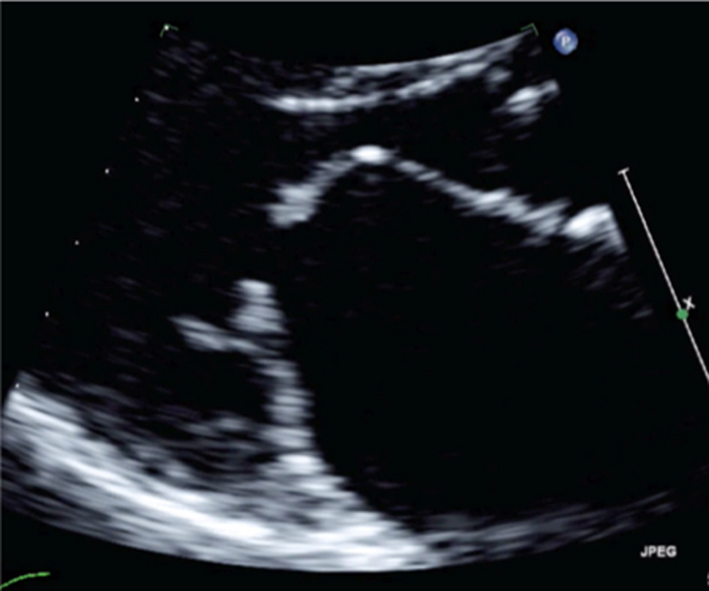
PLAX	Image 1 Visual assessment of annular calcification, leaflet thickness and excursion	Measure leaflet tip thickness in mid-diastole and describe the degree of leaflet restriction Describe the extent of annular calcification and how far this extends into the posterior leaflet Report features suggestive of aetiology
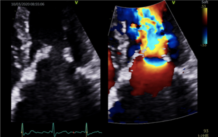
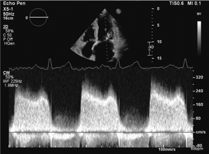
A4C	Image 2 Mean pressure gradient	Zoom on the MV in the A4C view. Apply CFD to identify the centre of the MV orifice and direction of flow.
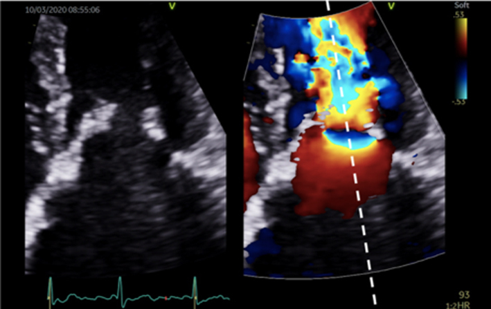
	Image 3	Place the cursor through the centre of the orifice and aligned with the flow (tip: place the cursor through the highest PISA seen within the LA
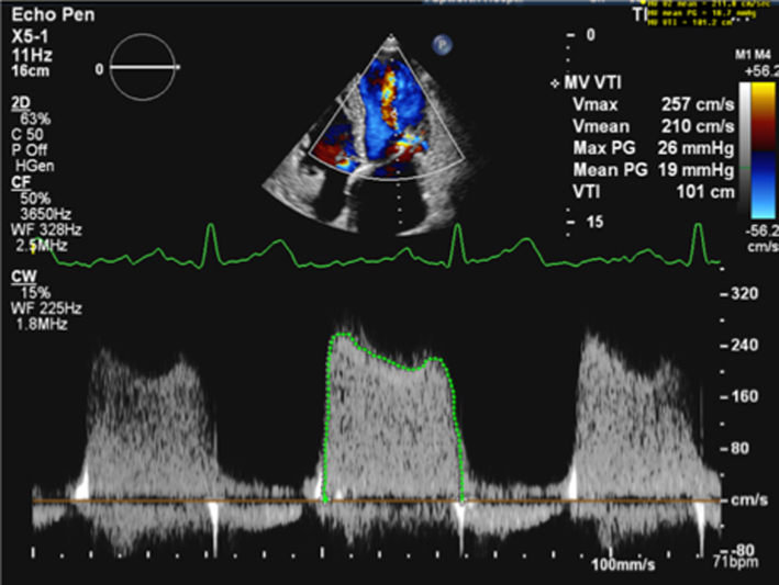
	Image 4	Enter CW Doppler mode, optimise and record several beats. Trace the MV signal.
	Image 5	Poorly optimised images can lead to overestimation of the Doppler signal and, therefore, overestimation of the mean pressure gradient
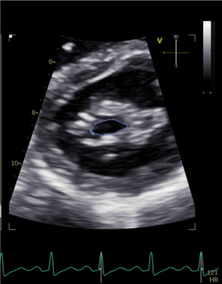
	Image 6 2D Planimetry	In the PSAX view at the level of the MV, find the plane of the leaflet tips by scanning back and forth through the valve. Once in the correct plane, zoom on the valve and freeze. Scroll through the loop to find the point in diastole when the leaflet excursion is at its greatest. Trace along the blood-tissue interface of the leaflet tips (tip: although it is not recommended to trace around CFD overlaid onto the MV orifice, applying CFD can help identify orifice geometry and therefore guide more accurate measurement).
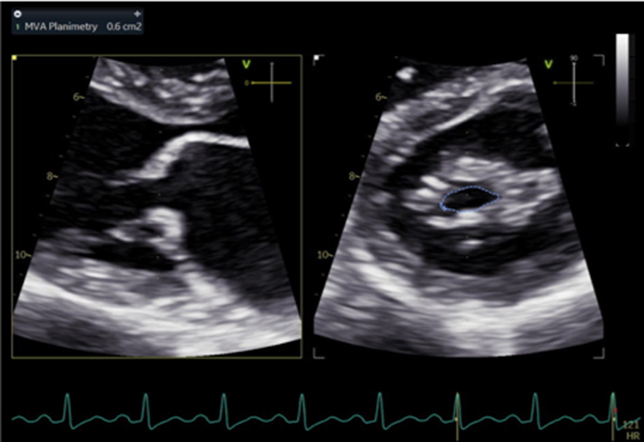
Parasternal window	Image 7 3D – orthogonal plane imaging	Orthogonal plane imaging can help ensure that orifice planimetry is performed at the leaflet tips. Place the cursor at the level of the MV tips and enter orthogonal plane imaging to demonstrate the MV orifice; the MVA can then be traced. Limitation: Off axis imaging in the PLAX plane will lead to an oblique image of the MV and overestimation of the MVA in the orthogonal view.
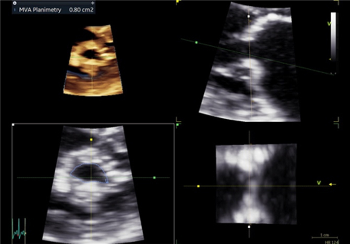
PLAX	Image 8/9 3D volume imaging	In the PSAX view at the level of the MV, acquire a 3D zoom dataset; this should be optimised to include the entire mitral annulus but no more than a few millimetres above leaflet height. Acquire the 3D volume dataset. Using multi-plane reconstruction, crop the dataset to identify three planes of the valve. Scroll through the loop to find the point in diastole when the leaflet excursion is at its greatest. Adjust the plane of view that is en-face with the valve to achieve parallel alignment with the orifice. Trace along the blood-tissue interface of the leaflet tips to measure MVA.
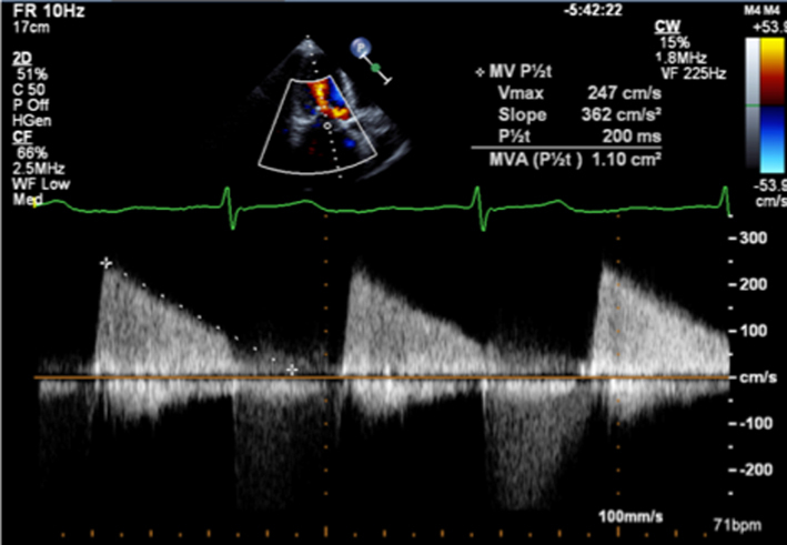
A4C	Image 10 P½t	Apply CFD to the A4C to identify the MV orifice. Place the cursor through the centre of the orifice (tip: when a PISA is seen within the LA, ensure the cursor is positioned through its highest point). Enter CW mode, the signal can be optimised by: ensuring parallel alignment with the trans-mitral flow, adjusting the velocity scale to maximise the Doppler signal size. Optimising signal gain and reject to reduce transit-time artefact. Measure the deceleration slope from the peak of the signal to the baseline of 0 cm/s. If the E signal is bi-modal, ignore the initial descent and measure the slope from mid-diastole onwards When the patient is in AF, measure according to the described guidance.
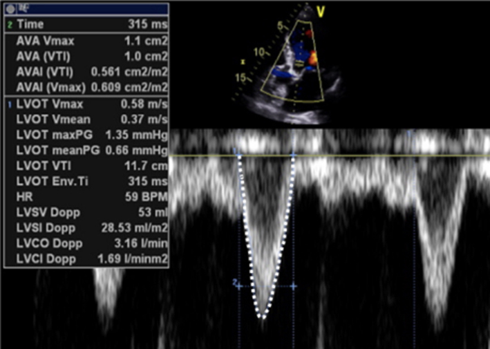
PLAX and apical views	Image 11 Continuity estimates	LV SV is calculated at the level of the LVOT by multiplying the CSA by LVOT PW VTI (tip: assuming circular geometry of the LVOT often leads to underestimation of SV and consequently MVA. SV can also be estimated by 2D biplane and 3D estimates of LV EDV and ESV, similar limitations of AR and MR apply however) Apply CFD to the A4C to identify the MV orifice.
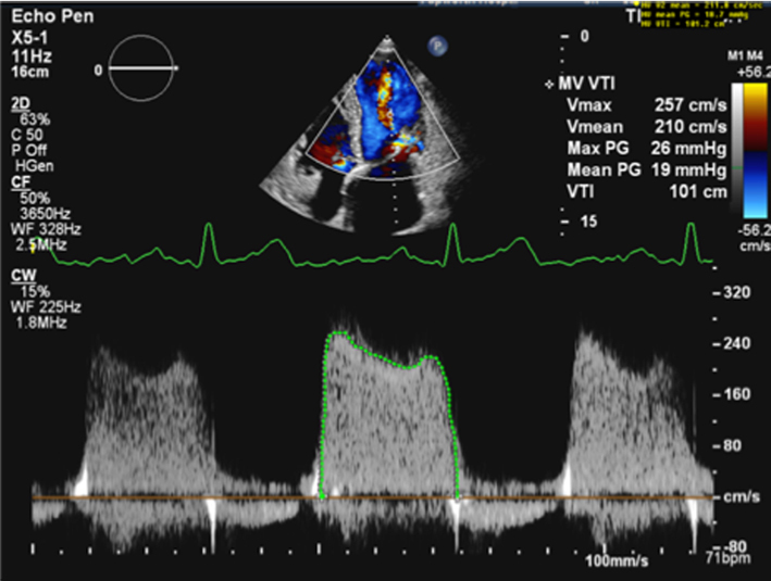
	Image 12 Continuity estimates	Place the cursor through the centre of the orifice and align with flow (tip: when a PISA is seen within the LA, ensure the cursor is positioned through its highest point). Enter CW Doppler mode and optimise the signal. Trace the MV signal.
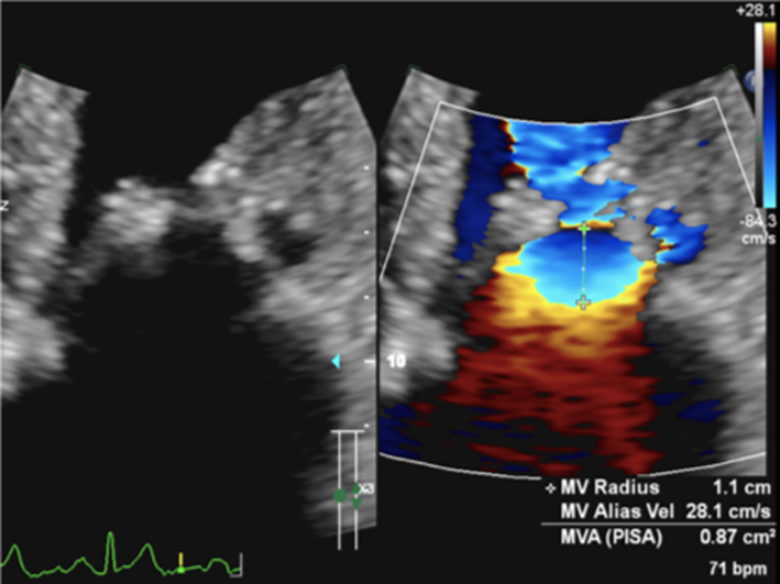
A4C	Image 13 PISA estimates of MVA	Zoom on the MV in the A4C view. Apply CFD and adjust the baseline in the direction of flow (tip: a lower Nyquist limit is more obvious when returning to normal CFD assessment and avoids acquiring the remainder of the study at a lower alias velocity). Freeze the image and scroll through to mid-diastole. Measure the PISAr from the point of the leaflet tips to the greatest radius.
	Image 14	Supress CFD and measure the angle of the atrial surface of the MV. This measure requires appropriate software. Unfreeze the image and place the cursor through the centre of the orifice (tip: place the cursor through the highest PISA radius) Enter CW mode and optimise the signal according to the guidance above. Trace the MV signal.