Table 5.

Guide to 2D image acquisition in mitral regurgitation

View	Measure or image	Explanatory note	Image
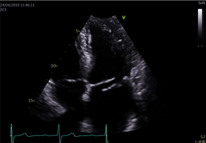
All views	Image 1 2D anatomy that is suggestive of severe MR	Report a flail leaflet, scallop or leaflet tip if part of the leaflet points towards the upper left atrium in systole (eversion).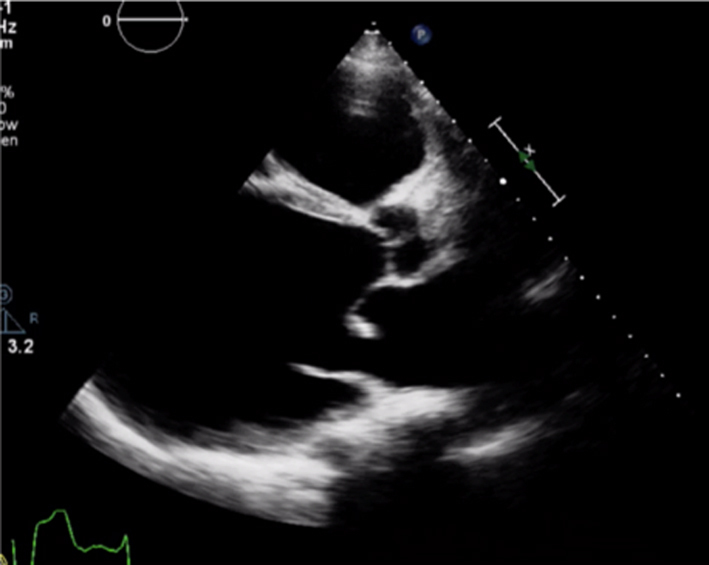
	Image 2 Coaptation defect	Describe clear coaptation defects and the location. Comment on which leaflet is affected, how extensive and which scallop. There will be severe regurgitation. Assess both papillary muscles and chordae for ruptures. To review the subvalvular apparatus, use all views available Report related findings according to suspected clinical aetiology, for example, regional wall motion abnormalities and left ventricle function in myocardial infarction, vegetations in endocarditis. Report MAD when seen.
	Image 3 Coaptation defect
	Image 4 Mitral annular disjunction
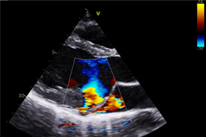
All views	Image 5 CFD PLAX	Optimise CFD settings (see BSE Minimum Dataset (7)). Adjust the lateral CFD Region of Interest (ROI) to include 1 cm of the LV on the left lateral border and the roof of the LA on the right lateral border (7). The CFD ROI height should not extend beyond the anterior and posterior LA walls. Simultaneous MV and AV CFD assessment should not be performed. Eccentric jet PISA should be measured in the view that the greatest radius is seen
	Image 6 PLAX PISA
PSAX	Image 7 CFD MV leaflet tips level	Apply CFD to the short-axis view of the MV to identify the location and extent of the regurgitant orifice along leaflet coaptation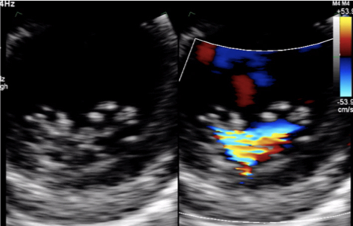
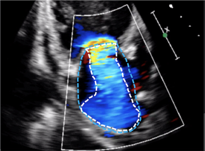
All apical views	Image 8 CFD assessment of MR	Ensure that the CFD box is optimised to demonstrate the whole MR jet, but that temporal resolution is maintained by not extending the CFD box beyond what is required to view the regurgitant jet. Describe the jet characteristics: direction, width, how far it extends into the LA.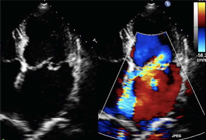
	Image 9 MR CFD	Calculate jet area by tracing both the MR jet and the LA area. Jet area >50% of LA area suggests severe MR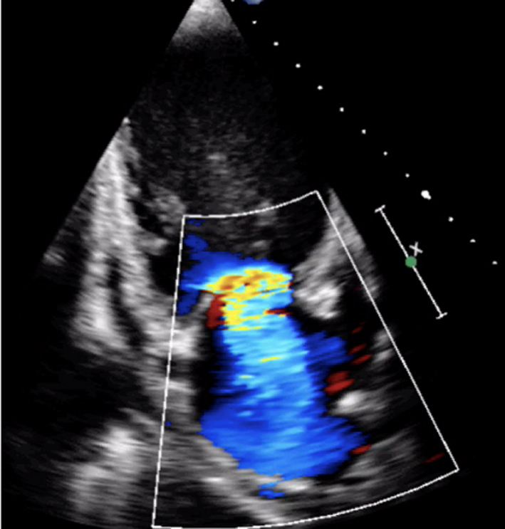
	Image 10 MR jet area
All views	Image 11 MR CW	Assess CW density for a qualitative assessment of MR Place the cursor through the PISA and VC. Enter CW mode and optimise, ensuring that the full MR signal is visualised below the baseline and that the forward flow signal is visible above the baseline. A faint CW Doppler signal is suggestive of trace-mild MR; CW signal density increases as MR becomes more severe such that severe MR CW is of similar density to the diastolic forward flow density (33). Limitation: Poor alignment with eccentric jets can lead to incomplete spectral Doppler signals or discrepant signal density for the degree of regurgitation.
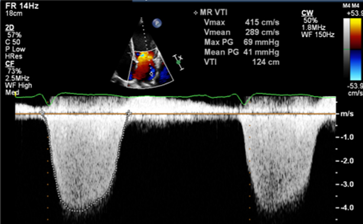	Image 12	Report density and signal waveform, including shape (triangular vs parabolar) and pre-systolic components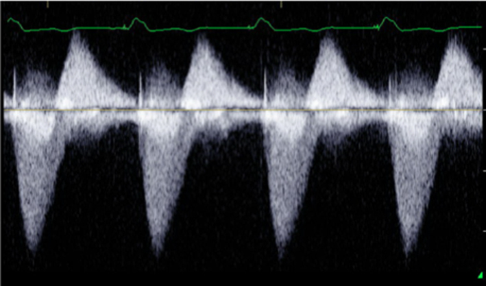
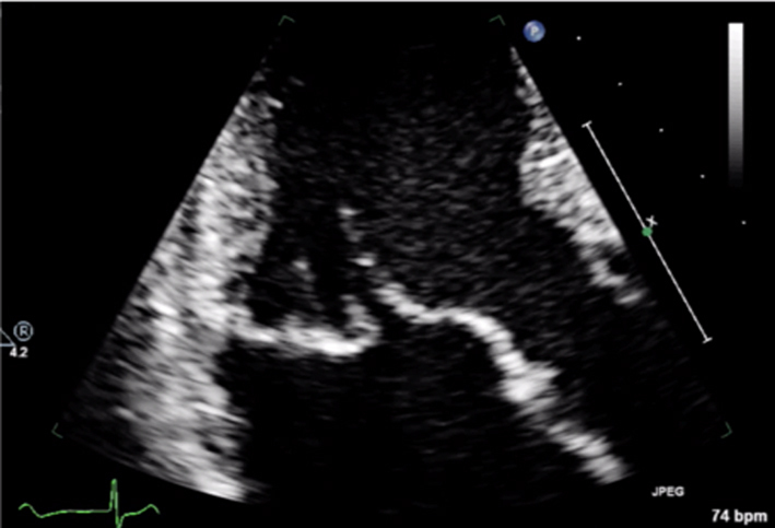
	Image 13 How to measure vena contracta
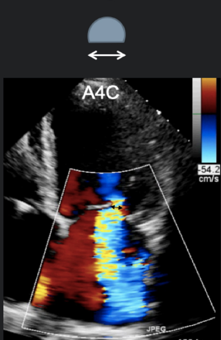
	Image 14 A4C VC measure	Obtain a clear view of the colour flow through the mitral valve in PLAX, A4C or A2C viewsIf necessary, scan along the commissural line to identify the regurgitant orifice and that the PISA, VC and jet expansion are demonstrated. Zoom in on the colour flow through the mitral valve. Record a loop and scroll through to identify the image with maximal flow through the valve. The VC is the narrowest region of the regurgitant jet (usually just above the valve in the left atrium). Report the average diameter. Single plane diameter ≥0.7 cm or biplane ≥0.8 cm suggests severe MR. Limitations of VC: This method is simple and thought to be independent of haemodynamics, driving pressure, and flow rate. However, low colour gain, poor acoustic windows, and inability to assess multiple jets can underestimate the VC. A high colour gain, irregular shape of jet, or atrial fibrillation can lead to overestimation
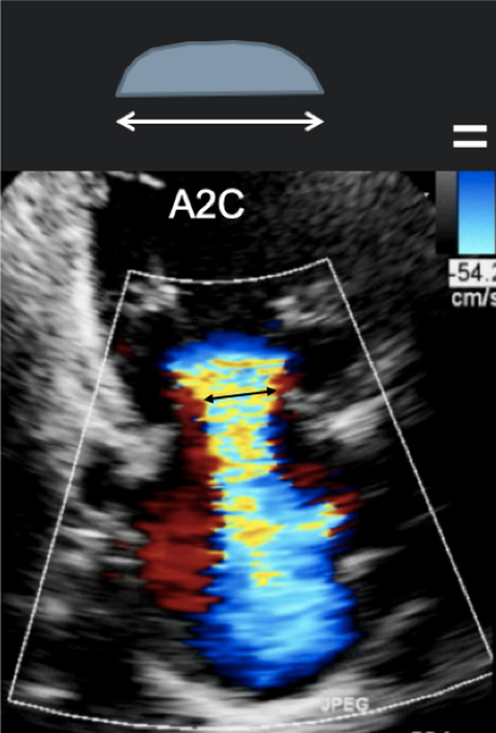
	Image 15 A2C VC
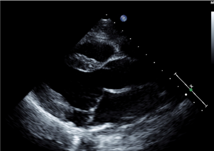
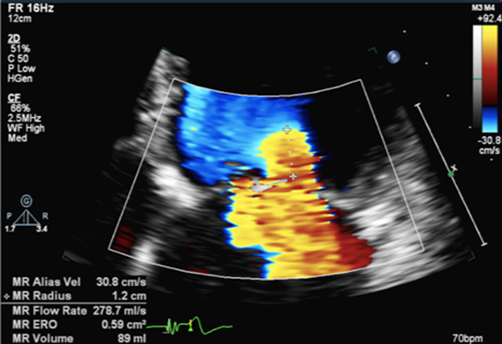
	Image 16 PISA measures for MR	Zoom on the mitral valve and apply CFD. Reduce the Nyquist limit to between 20 and 40 cm/s (tip: a lower Nyquist limit is more obvious when returning to normal CFD assessment and avoids acquiring the remainder of the study at a lower alias velocity). Once the PISA is clearly seen, gently tilt the probe back and forth to scan through the PISA and identify the greatest radius. Freeze and scroll through the image to the point of the greatest radius, bearing in mind that the PISA radius can be dynamic according to mechanism.
	Image 17 PISA measure in modified PLAX	Measure from the leaflet tips to the maximum PISA height (tip: once the height has been measured, supress CFD from the image to ensure that the PISAr measure is from the leaflet surface. Alternatively, utilse colour compare/simultaneous CFD and 2D imaging.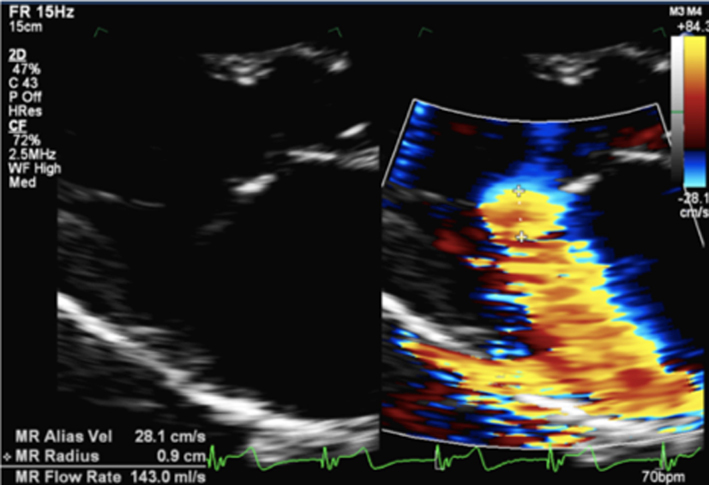
	Image 18 CF M-Mode to identify dynamic PISAr. CW Doppler demonstrating late systolic MR	Once the radius has been measured, unfreeze the image and place the cursor through the centre of the orifice (tip: place the cursor through the highest PISA radius and VC). Enter CW mode and optimise the signal according to the guidance above.
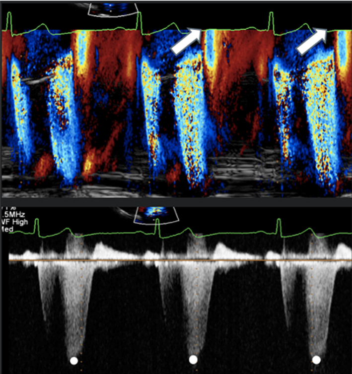	Image 19 End systolic CW trace	Trace the MR signal. Aim to measure the MR CW signal during a similar R-R as that of PISA measure.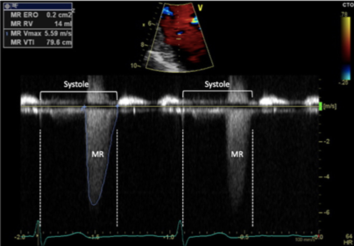
	Image 20 CFD M-Mode late systolic MR	Early or late systolic MR jets should be traced accordingly. Estimate of EROA alone, by measuring just MR Vmax, is not recommended in this scenario and can lead to overestimation of MR severity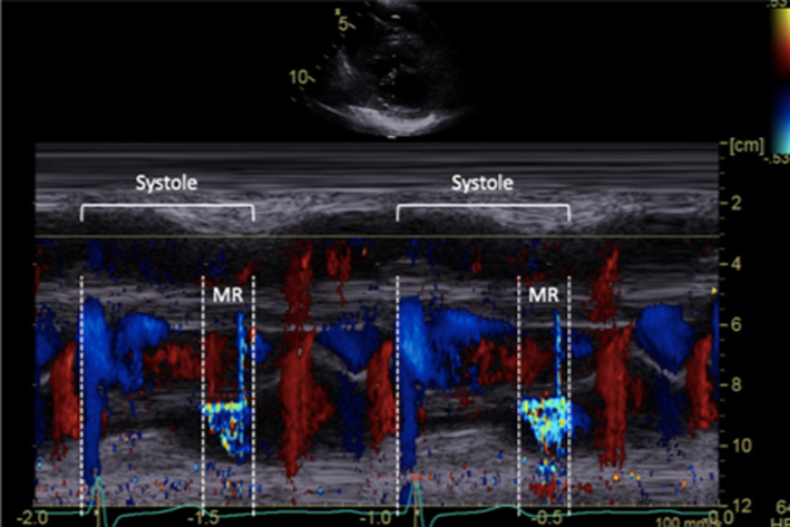
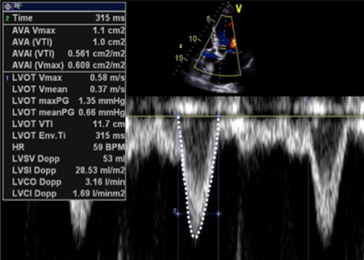
	Image 21 Continuity for MR	Calculate the LV SV at the level of the LVOT according to the guidance above. Zoom on the MV in the A4C view and apply CFD. Place the cursor at the leaflet tips and enter PW mode. Optimise the PW signal. Freeze the image and trace the Doppler signal.
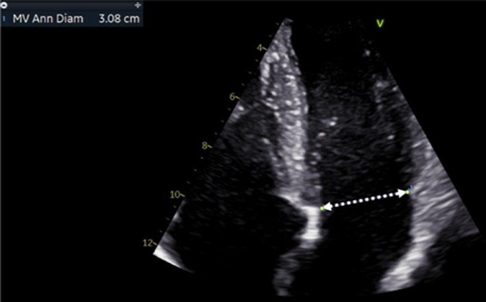
	Image 22	Zoom on the MV in the A4C view, ensure that the full annular diameter is included in the image. Freeze the image. Scroll to a point in early- to mid-diastole, measure the annular diameter.
	Image 23	Perform the continuity assessment of calculating SV at both sites. Subtract the LVOT SV from the MV SV, the difference is the estimation of regurgitant volume (limitations apply, see the ‘Continuity equation’ section)
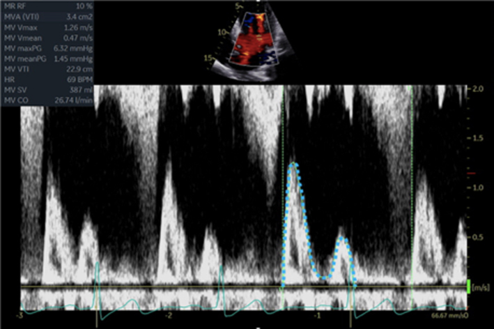
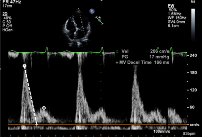
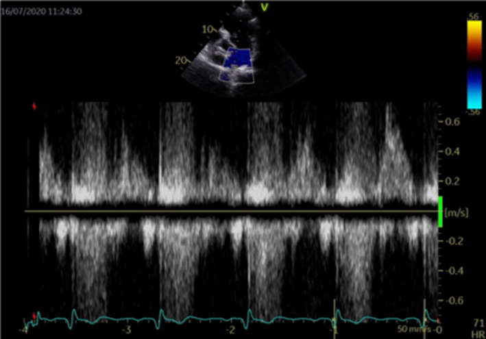
	Image 24 Transmitral flow velocity	Place sample volume (1–3 mm) at level of the MV leaflet tips in diastole. Use of CFD can help to align with the centre of trans-mitral flow. Measure at end expiration Emax: peak velocity in early diastole Amax: peak velocity in late diastole (after P wave) DT: Flow deceleration time from peak E wave to end of E wave signal (25). E wave > 1.5 m/s is suggestive of severe MR in the absence of high-flow states and MS. An E/A ratio < 1 is nearly certainly indicative of non-severe MR.
	Image 25 PV flow reversal	Superior angulation of transducer and use of CFD can help locate the pulmonary veins. The right lower pulmonary vein (RLPV) is most likely adjacent to the atrial septum in the A4C view, with the right upper pulmonary vein likely to be visualised in the A5C view (39).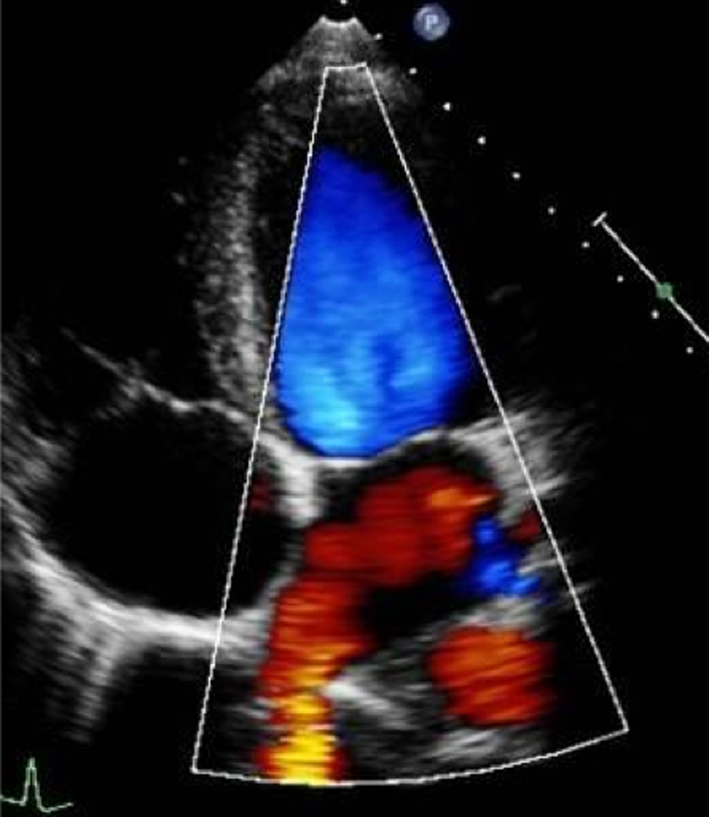
	Image 26 Pulmonary vein flow	Place sample volume (1–3 mm) 1–2 cm into the vein. Use fast sweep speed (50–100 mm/s). Measure at end expiration. PulV S: peak velocity in early systole (after QRS) PulV D: Peak velocity in early diastole.
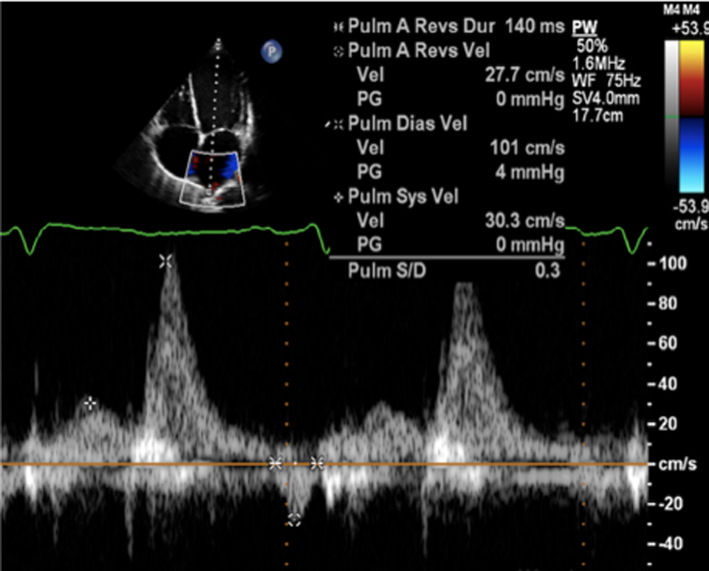	Image 27 Flow reversal in pulmonary vein	Report systolic flow reversal or blunted S wave. Limitations: any pathology that increases left atrial pressure can blunt PulV flow, LV diastolic dysfunction should be excluded before PV flow is reported. Because PulV S flow reversal has low sensitivity for identifying severe regurgitation, its absence does not exclude severe MR.
	Image 28A LV size and systolic function	Simpsons biplane method of discs should be used routinely to assess LV size and LVEF.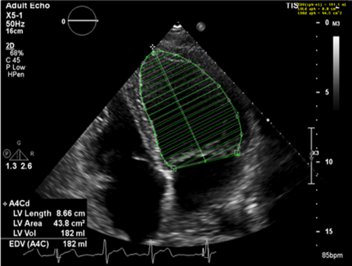
	Image 28B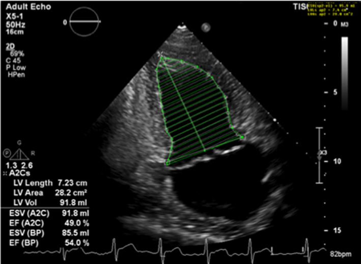
	Image 29	Due to the superior accuracy of volume estimation, 3D LV volume and EF is recommended for serial assessment of MR.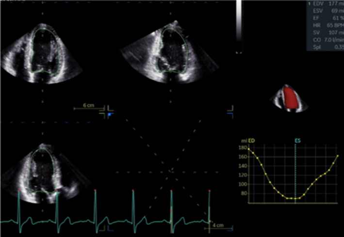
	Image 30	Strain may be helpful in identifying subclinical LV dysfunction in the setting of serial echocardiograms and may help determine appropriate follow-up intervals or timing for intervention.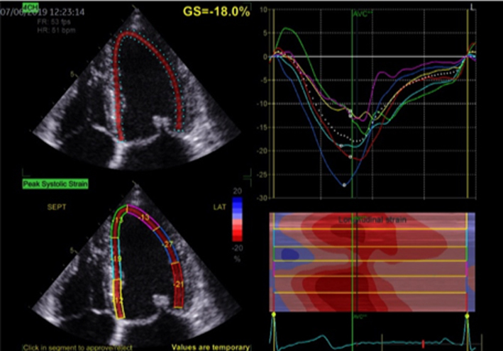
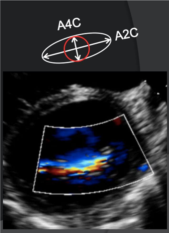
A4C and A2C	Image 31 LA volume	Biplane LA volume should be estimated using 2D imaging from the A4C and A2C views. As the long-axis dimensions of the LV and LA lie in different imaging planes, the standard apical views optimised for LV assessment do not demonstrate the maximal LA volume. The A4C and A2C images acquired for LA measurement should therefore be optimised to demonstrate the maximal LA length and volume at end-systole. Measurement is made using Simpson’s biplane method and according to the BSE Minimum Dataset (7). However, due to the superior reproducibility and without the need for geometric assumptions, 3D volume measures of the LA are recommended where possible.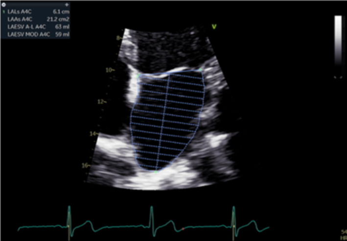
	Image 32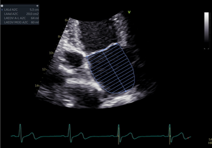
	Image 33 Peak TR velocity	Estimates of SPAP are important for timing MV intervention.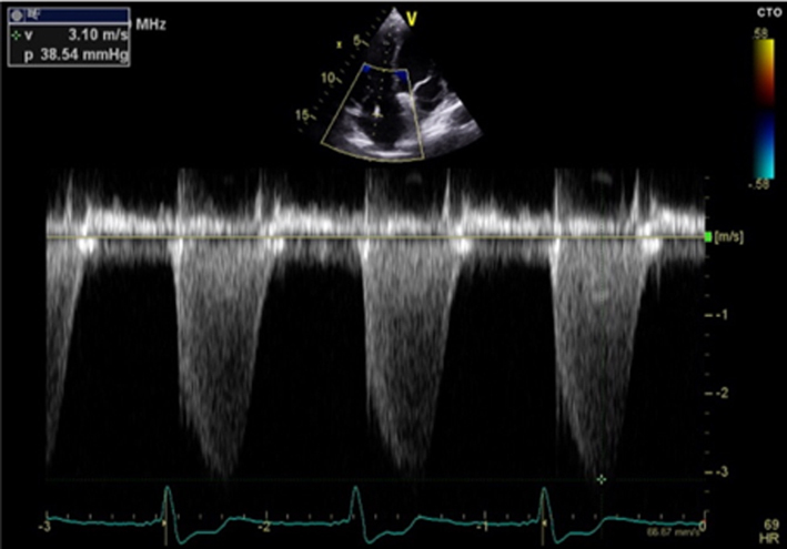