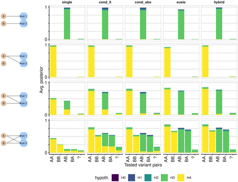
Fig 1. Average posterior probability distributions in simulated data.

The four classes of simulated datasets are shown in four rows, with the scenario indicated in the left hand column. For example, the top row shows a scenario where traits 1 and 2 have distinct causal variants A and B. Columns indicate the different analysis methods, with susie indicating SuSiE, cond_it indicating that coloc-conditioning was run in iterative mode, and cond_abo indicating it was run in “all but one” mode. For each simulation, the number of tests performed is at most 1 for “single”, or equal to the product of the number of signals detected for the other methods. For each test, we estimated which pair of variants were being tested according to the LD between the variant with highest fine-mapping posterior probability of causality for each trait and the true causal variants A and B. If r² > 0.5 between the fine-mapped variant and true causal variant A, and r² with A was higher than r² with B, we labeled the test variant A, and vice versa for B. Where at least one test variant could not be unambigously assigned, we labelled the pair “?”. The total height of each bar represents the proportion of comparisons that were run for that variant pair, out of the number of simulations run, and typically does not reach 1 because there is not always power to perform all possible tests. Note that because we do not limit the number of tests, the height of the bar has the potential to exceed 1, but did not do so in practice. The shaded proportion of each bar corresponds to the average posterior for the indicated hypothesis, defined as the ratio of the sum of posterior probabilities for that hypothesis to the number of simulations performed. Recall that H₀ indicates no associated variants for either trait, H₁ and H₂ a single causal variant for traits 1 and 2 respectively, H₃ and H₄ that both traits are associated with either distinct or shared causal variants, respectively. Each simulated region contains 1000 SNPs.