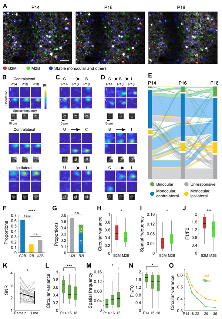
Figure 2: Longitudinal tracking of receptive field tuning properties from eye opening.

(A) Example field of view of GCaMP6s expressing pyramidal neurons that was repeatedly imaged on P14, P16, and P18. Neurons with tuning properties tracked across all three time points are colored with red, green and blue masks that represent those that were binocular at P14 and monocular afterwards (red; B2M), monocular at P14 and binocular afterwards (green; M2B), or stable monocular or with other trajectories (blue). Neurons without color masks (white) were not successfully tracked. Scale bar: 50 μm.
(B) Examples of receptive field tuning kernels from neurons that were stably monocular, responding solely to either the contralateral (C; upper two rows) or ipsilateral eye (I; bottom row). Below each kernel is an image of the cell.
(C) Examples of cells that gained responsiveness to an eye. Top: a cell that was monocularly driven by the contralateral eye at P14 and P16, but gains responsiveness to the ipsilateral eye at P18, thereby becoming binocular (C2B). Middle: a cell that was visually unresponsive at P14 but become solely responsive to contralateral eye stimulation at P16 and remains so at P18 (U2C). Bottom: a cell that was unresponsive at P14 but becomes solely driven by the ipsilateral eye at P16 (U2I).
(D) Examples of cells that shift their responsiveness from one eye to the other. Top: a cell that was solely responsive to the contralateral eye at P14, then binocular at P16, then solely responsive to the ipsilateral eye at P18. Middle: a cell that was binocularly responsive at P14, but solely responsive to the ipsilateral eye by P16 and again at P18. Bottom: a cell that was solely responsive to the contralateral eye at P14, but then became solely responsive to the ipsilateral eye thereafter.
(E) Sankey diagram plotting the functional trajectory of 741 neurons that were longitudinally imaged at P14, P16, and P18. Length of boxes at each day represents proportions of different groups. Cells are color coded retrospectively. For example, if a neuron ended up binocular at P18, it is color coded green.
(F) Proportion of binocular neurons that formed via conversion of neurons in P14-16 or P16-18 that were initially solely responsive to the contralateral eye (C2B, n=67), solely responsive to the ipsilateral eye (I2B, n=17), or unresponsive (U2B, n=26). Chi-square test for pairwise comparisons with Bonferroni correction; ****, p<0.0001 after the Bonferroni correction.
(G) Proportion of neurons solely responsive to the ipsilateral eye that formed from initially unresponsive neurons (U2I, n=63), or from neurons that were initially solely driven by the contralateral eye (C2I, n=35) or were binocular (B2I, n=16), and thus responsive to the contralateral eye (R2I). Chi-square test for pairwise comparisons.
(H) Circular variance of neurons that were binocular but became monocular (B2M, n=41) and of monocular neurons that became binocular (M2B, n=84). Black horizontal line, median; box, quartiles with whiskers extending to 2.698σ. Mann-Whitney U test; *, p<0.05.
(I) As in H, but for measures of spatial frequency preference; *, p<0.05.
(J) As in H, but for measures of response linearity; ***, p<0.001.
(K) Signal to noise ratio (SNR) of responses to each eye in binocular neurons prior to the loss of one eye’s responses (n=33). Gray, measurements for individual neurons; black, mean ± standard deviation. Mann-Whitney U test of SNR between remained and lost eye specific responses; *, p<0.05. Note: the SNR of the response of the eye that remained was stronger than that of the eye that was lost.
(L) Circular variance of binocular neurons measured at P14 (n=15), P16 (n=46), and P18 (n=84). Mann-Whitney U test between P14 and 18; ***, p<0.001. Note the gradual improvement in orientation selectivity with age.
(M) As in L, but for spatial frequency tuning; *, p<0.05.
(N) As in L, but for linearity. *, p<0.05.
(O) Plot of circular variance for binocular neurons (n=74, 220, 450, 417, 339) and neurons driven by the ipsilateral eye (n=147, 562, 1024, 931, 832) from eye opening until the end of the critical period at P36. Note the continual improvement with age.
