Strategies for feature extraction from structural brain imaging in lesion‐deficit modelling

Abstract

High‐dimensional modelling of post‐stroke deficits from structural brain imaging is highly relevant to basic cognitive neuroscience and bears the potential to be translationally used to guide individual rehabilitation measures. One strategy to optimise model performance is well‐informed feature selection and representation. However, different feature representation strategies were so far used, and it is not known what strategy is best for modelling purposes. The present study compared the three common main strategies: voxel‐wise representation, lesion‐anatomical componential feature reduction and region‐wise atlas‐based feature representation. We used multivariate, machine‐learning‐based lesion‐deficit models to predict post‐stroke deficits based on structural lesion data. Support vector regression was tuned by nested cross‐validation techniques and tested on held‐out validation data to estimate model performance. While we consistently found the numerically best models for lower‐dimensional, featurised data and almost always for principal components extracted from lesion maps, our results indicate only minor, non‐significant differences between different feature representation styles. Hence, our findings demonstrate the general suitability of all three commonly applied feature representations in lesion‐deficit modelling. Likewise, model performance between qualitatively different popular brain atlases was not significantly different. Our findings also highlight potential minor benefits in individual fine‐tuning of feature representations and the challenge posed by the high, multifaceted complexity of lesion data, where lesion‐anatomical and functional criteria might suggest opposing solutions to feature reduction.

Kasties et al. compared the suitability of different featurisation strategies in lesion‐behaviour modelling. They found no significant differences in model performance between voxel‐wise, atlas‐based region‐wise and componential featurisation. This demonstrates the general suitability of all three commonly applied feature representations in lesion‐behaviour modelling.

Abbreviations

CoC

centre of cancellation

CV

cross‐validation

PCA

principal component analysis

RBF

radial basis function

ROI

region of interest

SVR

support vector regression

MSE

mean squared error

1. INTRODUCTION

In cognitive neuroscience, mathematical models of the relation between post‐stroke deficits and structural brain imaging data are crucial both in basic and translational research. In basic research, lesion‐deficit models are used to map the functional architecture of the human brain. The most popular method to date, voxel‐based lesion‐behaviour mapping (Bates et al., 2003; Rorden & Karnath, 2004), maps the neural correlates of post‐stroke behavioural abnormalities using mass‐univariate models for each voxel individually. Recently, multivariate modelling of stroke imaging data became popular, either applied on voxel‐wise imaging data (e.g., Ivanova, Herron, Dronkers, & Baldo, 2020; Pustina, Avants, Faseyitan, Medaglia, & Coslett, 2018; Sperber, Wiesen, & Karnath, 2019; Xu, Rolf Jäger, Husain, Rees, & Nachev, 2018; Zhang, Kimberg, Coslett, Schwartz, & Wang, 2014), or region‐wise data (e.g., Achilles et al., 2017; Smith, Clithero, Rorden, & Karnath, 2013; Yourganov, Smith, Fridriksson, & Rorden, 2015). In translational research, lesion behaviour models have the potential to predict post‐stroke outcome and guide individualised rehabilitation and care. For this application, univariate models are only rarely used (e.g., Feng et al., 2015), and multivariate algorithms dominate the field (e.g., Hillis et al., 2018; Hope, Seghier, Leff, & Price, 2013; Loughnan et al., 2019; Rondina, Filippone, Girolami, & Ward, 2016; Rondina, Park, & Ward, 2017; Siegel et al., 2016; Xu et al., 2018).

Structural imaging data in lesion‐deficit modelling are commonly either binary maps identifying lesioned tissue or continuous maps indicating a voxel's probability of being lesioned. In the process of spatial normalisation, these data are warped to a common imaging space (see de Haan & Karnath, 2018), resulting in voxel‐wise lesion images. In the commonly used 1 × 1 × 1 mm³ imaging space, the cerebrum makes up more than a million voxels. Neighbouring voxels in this high‐dimensional data space often carry similar or even the same information, that is, pairs of voxels might exist that are always damaged together in a given population of stroke patients. This vast amount of highly correlated input features poses a challenge to any high‐dimensional modelling algorithm, exacerbated by the typically small sample sizes in the field, which rarely exceed 200 patients.

While it is common in the field to use voxel‐wise data, two feature extraction strategies to handle such high‐dimensional imaging data exist. Voxel‐wise data is often either merged into (i) atlas‐based region‐wise data or (ii) data‐driven feature‐reduced, componential data. Both approaches aim to transform the imaging data into a lower‐dimensional data space. This is achieved ideally by meaningfully merging voxels with similar information into a new feature.

Following the region‐wise strategy, brain regions are defined by a brain atlas located in the same imaging space as the lesion map. The overlap of the lesion map with each atlas‐defined region is then utilised as a new feature, for example, by computing for each atlas region and patient the so‐called lesion load, the proportion of lesioned voxels. This approach has been widely used, especially with morphological brain atlases (e.g., Achilles et al., 2017; Hope et al., 2013; Rondina et al., 2016; Smith et al., 2013; Toba et al., 2017; Yourganov et al., 2015). Merging voxels in a neurobiologically meaningful way is a critical aspect of feature reduction. It allows us to capture the available information better and enhance our understanding of the brain (Eickhoff, Constable, & Yeo, 2018). Consequently, it might be advantageous to use a functional instead of a morphological brain parcellation when predicting impairments in normal function from lesion topography. Recent state‐of‐the‐art brain atlases provide brain parcellations based on different functional criteria (e.g., Fan et al., 2016; Glasser et al., 2016; Joliot et al., 2015). These allow merging information of all voxels that are part of the same functional area meaningfully into a single feature.

Following the data‐driven feature reduction strategy, the dimensionality of voxel‐wise lesion data is reduced by unsupervised learning algorithms such as principal component analysis (PCA; e.g., Siegel et al., 2016; Salvalaggio, De Filippo De Grazia, Zorzi, Thiebaut de Schotten, & Corbetta, 2020; Zhao, Halai, & Lambon Ralph, 2020; Ivanova et al., 2020). The underlying rationale is that voxel‐wise lesion information is highly correlated between voxels due to the typical anatomy of lesions (Sperber, 2020; Zhao et al., 2020). In other words, many voxels in the brain are systematically damaged together by brain lesions and their informational content is highly similar. Hence, these voxels might be merged into a single feature without sacrificing information. In summary, data‐driven feature reduction allows integrating features according to their lesion‐anatomical information.

Both region‐wise functional and lesion‐anatomical componential feature reduction strategies bear the potential to counter the burden of dimensionality in lesion‐deficit models and improve a model's predictive power. However, both approaches can lead to conflicting feature reduction solutions, for example, if two voxels are functionally highly correlated (i.e., they are both parts of the same functional module), but their lesion‐anatomical similarity is low, or vice versa (Sperber, 2020). To date, a systematic comparison of both approaches is still missing.

To our knowledge, so far, only region‐wise lesion load models and voxel‐wise models were directly compared in a study that predicted post‐stroke motor outcome from imaging data (Rondina et al., 2016). They found voxel‐wise models to outperform any region‐wise model markedly. However, they did not utilise a brain parcellation of functional regions but a morphological atlas, which might have limited region‐wise modelling performance.

In the current study, we systematically compared voxel‐wise, atlas‐based region‐wise and data‐driven dimensionality reducing strategies to represent structural lesion data in modelling post‐stroke deficits. We modelled acute behavioural post‐stroke measures of spatial neglect and paresis of the upper limb with high‐dimensional, machine‐learning‐based algorithms. The study's main objective was to identify the data representation strategy that provided the best predictive model performance. A secondary, exploratory objective was to compare different brain atlases' suitability in lesion‐deficit modelling.

2. METHODS

2.1. Study design—general overview

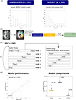
The study included multiple steps (see Figure 1 for schematic illustration), which can be outlined as follows: Two common post‐stroke symptoms were assessed in two different samples. We created normalised binary lesion maps from structural imaging and extracted features either as region‐wise lesion load using five different brain atlases or by data‐driven feature reduction via PCA. To provide a level playing field for comparisons, we compared all feature representation strategies (voxel vs. region vs. PCA components) for the same voxels, that is, voxel‐wise data and derived PCA components always included only voxels that were labelled in the brain atlas, but not voxels in unlabelled areas. We fit support vector regression models to predict behavioural scores based on the three different feature representations and used a repeated six‐fold nested cross‐validation (CV) to assess model performances. Furthermore, we calculated the permutation importance for principal components and ROIs and eliminated the least important features within the inner loop of the CV procedure. Generally, high‐dimensional datasets usually include many features that carry non‐relevant information. Models might be overfitted to non‐relevant features, decreasing model performance. Therefore, this condition allowed an evaluation of different feature representation strategies in a potentially more effective way more relevant to clinical applications. Last, model performance was compared across conditions with non‐parametric statistical tests on the individual squared errors.

FIGURE 1.

Study design. (a) Datasets and distributions of behavioural scores. The mean CoC was root‐mean‐square‐transformed to obtain a more even distribution. (b) Extraction of features from binary lesion maps. (c) An epsilon—SVR with radial basis kernel (RBF ε‐SVR) was used to model the relation between features and behavioural scores. The plot shows the repeated nested cross‐validation procedure schematically: the inner loop serves for hyperparameter optimisation on a validation set (Val) and the outer loop for testing the model performance of a trained model (on the training data, “Train”) on held‐out test sets (Test). (d) We assessed model performance using the squared correlation coefficient of predicted and measured behavioural scores and compared models with non‐parametric tests on squared errors. For more information, see Section 2.1. Histograms represent the real distributions of behavioural scores. The other graphs shown are exemplary and based on simulated data

2.2. Patient recruitment and behavioural assessment

Neurological patients with first‐ever cerebral, unilateral stroke were recruited at the Centre of Neurology at the University Clinics Tübingen. Only patients with a confirmed stroke and a clearly demarcated, non‐diffuse lesion visible in CT or MRI were included. The recruitment involved two different samples: a sample of 203 acute right‐hemisphere stroke patients tested for spatial neglect (as reported in Wiesen, Sperber, Yourganov, Rorden, & Karnath, 2019) and a sample of 102 acute unilateral stroke patients tested for hemiparesis of the contralesional upper limb. For demographic data, see Tables S1 and S2. The study was performed in accordance with the revised declaration of Helsinki and was approved by the local ethics committee. All patients or their relatives consented to the scientific use of collected data.

In the first sample, spatial neglect was assessed with the letter cancellation task (Weintraub & Mesulam, 1985) and the bells test (Gauthier, Dehaut, & Joanette, 1989) on average 4.4 days (SD = 4.0) after stroke onset. Both tasks are pen and paper tests that consist of target items scattered among distractors on a horizontal sheet of paper. They were presented on a table in front of the patient and centred along the patient's sagittal midline. The patient was instructed to mark all target items, and tasks were continued until the patient had confirmed their completion twice. Task performance was evaluated by calculating the centre of cancellation (CoC; Rorden & Karnath, 2010), a continuous measure of the egocentric bias in spatial neglect. CoC scores of both tests were averaged to generate the study's final target variable. Any sub‐threshold negative mean CoC scores were set to 0 to obtain a linear scale representing neglect severity from 0 to 1. No patient suffered from a pathological supra‐threshold ipsilesional egocentric spatial bias. Additionally, CoC scores were square‐root transformed to yield a more uniform distribution, as piloting tests in another sample suggested that better model fits could be yielded when the target variable was transformed.

In the second sample, acute and chronic paresis of the contralesional upper limb was assessed with the British Medical Research Council scale on average 1.0 days (SD = 2.2; acute) and at least 50 and on average 423 days (SD = 440; chronic) after stroke onset. The British Medical Research Council scale ranges from 0 to 5 (0: no movement, 1: palpable flicker, 2: movement without gravity, 3: movement against gravity, 4: movement against resistance and 5: normal movement), and intermediate steps of 0.5 points were included. The final target variable was the average of distal and proximal ratings for the upper limb. Note that we found models on chronic hemiparesis scores to provide low quality with marked systematic biases in predictions. We judged comparisons between featurisation strategies for this measure not to be reliable and only report them in the Supporting Information.

2.3. Imaging and lesion delineation

Structural CT or MRI was obtained as part of clinical stroke protocols on average 3.5 days (SD = 4.6) after stroke onset in the sample tested for spatial neglect, and on average 2.1 days (SD = 2.7) in the sample tested for hemiparesis. In the case of multiple available imaging sessions, scans were chosen to be as acute as possible while clearly depicting lesion borders. For patients with MRI, areas of acute damage were visualised using diffusion‐weighted imaging in the first 48 hr after stroke onset and T2 fluid‐attenuated inversion recovery imaging later. If possible, these images were co‐registered with a high‐resolution T1 MRI to be used in the normalisation process.

Lesions were delineated on axial slices of the scans semi‐automatically using Clusterize (de Haan, Clas, Juenger, Wilke, & Karnath, 2015) or manually using MRIcron (https://www.nitrc.org/projects/mricron). Scans were warped into 1 × 1 × 1 mm³ MNI space using age‐specific templates from the Clinical Toolbox (Rorden, Bonilha, Fridriksson, Bender, & Karnath, 2012) and normalisation algorithms in SPM 12 (www.fil.ion.ucl.ac.uk/spm). Situation‐dependently we used either cost‐function masking or enantiomorphic normalisation to control for the lesioned area. Normalisation parameters were then applied to the lesion maps to obtain normalised binary lesion maps. Patients tested for spatial neglect all suffered from unilateral right hemispheric lesions; patients tested for hemiparesis had a unilateral stroke to either the left or the right hemisphere. In the present study, we did not aim to investigate possible hemisphere‐specific contributions to primary motor skills and, on the other hand, required a large sample with considerable informational content in the imaging features. Therefore, lesion maps of left hemispheric lesions in the second patient sample were flipped along the sagittal mid‐plane so that all lesions were depicted in the right hemisphere. This step reduces variability between subjects' lesion locations and increases the usable variance in individual imaging features. Overlap topographies of all lesions are shown in Figure S1 and the online materials at https://doi.org/10.17632/34rwd5vb2h.2.

2.4. Brain atlases

We chose five brain atlases, each parcellated based on different morphological or functional criteria. (a) The AAL3 , the most recent version of the popular automated anatomical labelling atlas (Rolls, Huang, Lin, Feng, & Joliot, 2020), a single‐subject morphological atlas with 166 areas; (b) the AALnbl , a combination of the AAL3 with the natbrainlab white matter atlas (32 white matter tracts; Catani & Thiebaut de Schotten, 2008); (c) the atlas of intrinsic connectivity of homotopic areas ( AICHA ), containing 192 homotopic functional region pairs (Joliot et al., 2015); (d) the Brainnetome atlas BN246 (Fan et al., 2016), a multimodal atlas containing cortical and subcortical grey matter (246 areas), and (e) a multimodal parcellation ( MMP ) as created and described in Pustina et al. (2018). The latter atlas was based on the multimodal surface‐based parcellation by Glasser et al. (2016). Pustina et al. (2018) transferred this atlas to volumetric MNI space, dilated parcels to include small portions of subcortical white matter below each parcel, and extended the atlas by subcortical regions taken from the BN246 (Fan et al., 2016) and the white matter JHU atlas (Hua et al., 2008). Left‐hemispheric and cerebellar brain regions were excluded from all atlases. We also provide a parcellation‐free analysis of our data in the Supporting Information.

2.5. Feature extraction

We extracted three different types of features from each patient's binary lesion image subsequently referred to as lesion load, voxels and principal components. Importantly, in each analysis iteration, we first chose an atlas and identified all voxels covered by the atlas, excluding all unlabelled voxels (e.g., subcortical white matter areas in a purely cortical atlas). Accordingly, the underlying data was the same for all three feature types (all voxels contained in the parcellation), which makes feature representations comparable to each other. Lesion load is the proportion of damaged voxels within each atlas region, resulting in a scalar between 0 and 1 per atlas region of interest (ROI). In the AALnbl atlas, we extracted the lesion load of all areas delineated by each atlas, disregarding potential overlaps of ROIs. Lesion load was calculated per atlas ROI and entered into a matrix of patients × ROIs per atlas. Additionally, we ensured that the included ROIs carried a usable amount of variance and removed those not damaged in at least 5% of all lesions. Correcting for minimal lesion affection closely resembles procedures in lesion‐behaviour mapping, where such criteria are commonly utilised to remove areas that can be considered outliers regarding their anatomical information (Sperber & Karnath, 2017).

Voxel‐wise features 0 (normal) and 1 (lesion) were then extracted from all retained atlas regions and entered into an m‐by‐n matrix (without considering any region label), where m is the number of patients and n the total number of voxels within a particular atlas. Voxels from overlapping areas in the AALnbl atlas were only extracted once. The resulting voxel matrix underwent PCA. In PCA, the features' covariance matrix is calculated, and a singular value decomposition is performed to find the subspace that explains the largest variance in the data. To assess the number of principal components that should be retained from the data, we implemented Horn's Parallel Analysis (Horn, 1965). Following this objective strategy to identify significantly relevant components, we resampled and diagonalised 1,000 random correlation matrices of the same dimensions as the original data. This yielded a distribution of eigenvalues, from which we estimated a 95% confidence interval and retained those eigenvalues that exceeded the upper confidence limit. See Figure S2 for an example scree plot and the online materials for the complete set of scree plots.

2.6. Data modelling—support vector regression and hyperparameter optimisation

We used high‐dimensional machine‐learning models to predict continuous behavioural scores from features extracted from the patients' MRI or CT images. Epsilon—support vector regression (ε‐SVR; Smola & Schölkopf, 2004) is such a supervised learning algorithm suited for predicting continuous dependent variables. Its goal is to obtain a function under the condition that the predicted values are within a set accuracy ε from the true score. In other words, we do not accept errors larger than ε but disregard deviations that are smaller than this. We fit an ε‐SVR with a radial basis function (RBF) kernel for each atlas and feature type in a repeated six‐fold nested CV regime. The non‐linear RBF kernel was reported to outperform linear kernels in lesion behaviour modelling (Hope, Leff, & Price, 2018; Zhang et al., 2014). We used functions provided by libSVM Version 3.24 (Chang & Lin, 2011; https://www.csie.ntu.edu.tw/~cjlin/libsvm/) running in a MATLAB R2020a environment.

Following the recommendations by Hsu, Chang, and Lin (2003), we first linearly rescaled all the features to the range [0, 1] before fitting models. We used the default ε of 0.1 in all models concerning the hemiparesis data and ε = 0.01 in the neglect sample to adapt to the scaling of the outcome variable. We generated six random folds of approximately equal size where one was held out as a test set in each outer loop iteration, whereas the model was fit on the remaining five folds (which together comprised the training set). The inner loop served for soptimising hyperparameters cost (C) and γ on each training set in an automatic grid search with a five‐fold CV.

Each model was evaluated within the inner loop in terms of its mean squared error (MSE) and mean squared correlation coefficient (R ²) across all five folds. The squared correlation coefficient is derived from the Pearson correlation coefficient between the values predicted by the model and the observed values in the test set (see formula 1 in the Supporting Information). We chose C‐ and γ‐ranges according to suggestions by Hsu et al. (2003), with C = [2⁻⁵, 2⁻³, …, 2¹⁵] and γ = 2⁻¹⁵, 2⁻¹³, …, 2³]. We repeated the five‐fold CV with every possible parameter combination to find the combination that sminimised MSE. If several equally small MSEs were found within the grid, we consulted R ² and extracted the combination that additionally smaximised this metric among the potential candidates.

The optimal hyperparameters were used to re‐train the model, and predictions were made on the held‐out test set. The outer loop was iterated six times to obtain a prediction for every patient in the set. The whole nested CV procedure was repeated five times with a random re‐shuffle of folds at each repetition. In total, this yielded five predictions per patient, which were averaged to mitigate the variance induced by random shuffling (Arlot & Celisse, 2010; James, Witten, Hastie, & Tibshirani, 2013; Varoquaux et al., 2017). We calculated the squared correlation coefficient between predicted and true behavioural scores and the squared error for each observation based on these averaged predictions. Importantly, repeated random splits were generated with the same random seeds for all models to ensure comparable models.

2.7. Data modelling—additional feature elimination

In lesion‐behaviour mapping, models including all (whole brain) data are common (e.g., Zhang et al., 2014). However, in translational applications, feature elimination, that is, only including highly informational features, could improve the model fit of clinically relevant predictions (Rondina et al., 2016). We assumed that training an SVR with only the most relevant features would improve the model's prediction accuracy and thus provide better means to evaluate the algorithm's real‐world application. Such endeavour is computationally demanding in high dimensional data, especially within a nested CV framework. Hence, we restricted feature elimination to lesion load and PCA representations, where a few dozen features were present each, compared to voxel‐wise data that contained up to over 700.000 features.

In a first step, we assessed the importance of individual features using a permutation approach originally formulated for random forests (Breiman, 2001) but can be similarly applied to other classification and regression problems (Fisher, Rudin, & Dominici, 2018; see Figure 2 for an illustration). It relies on disrupting an individual feature's association with the target variable by randomly shuffling it while leaving the other variables intact. Consequently, the loss of model performance induced by the permutation can be quantified in terms of the variable's permutation importance. This can be repeated for every variable in the data set. We calculated the variable importance of any given feature i as the ratio of the MSE under permutation of feature i versus the MSE of the model when all variables were left intact (Fisher et al., 2018; see Formula (2) in Supporting Information). A value above 1 indicates that the model relies on the variable for its predictions. However, there is no established threshold as to when to consider a variable ‘important enough’. Consequently, we sorted the variables according to their permutation importance and defined three subsets of different sizes, including only the variables with the largest importances.

FIGURE 2.

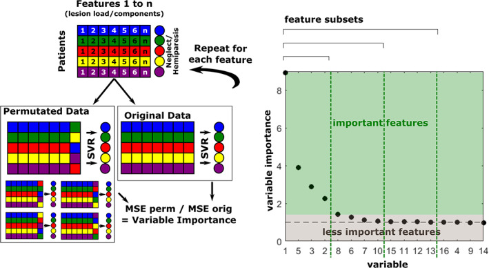
Schematic of the permutation‐based feature elimination. The left panel shows how variable permutation importance was calculated: for each feature, we assessed how permuting this feature would affect model performance compared to leaving the feature intact. Each variable was shuffled five times. The right panel shows an exemplary variable importance plot of 16 principal components that were labelled according to their occurrence in the original feature matrix. A feature can be regarded as important if variable importance is above 1. In the absence of a valid threshold for when to consider features ‘important enough’, three different subsets of features were retained, containing 25, 50 or 75% of the most important features. Graphs show exemplary simulated data

To implement this additional feature selection step in the six‐fold nested CV, we split the outer loop training set into two subsets containing two thirds and one‐third of training set observations, where the smaller sample served as a validation set. Hyperparameters were optimised for the larger set in a five‐fold CV grid search as described above, and a model with optimised C and γ was fit on the two‐thirds sample. Then, the reference loss (no shuffling) was obtained from the predictions made on the validation set. We consecutively resampled each feature without replacement and tested the model on the validation set after every permutation. We shuffled each feature five times and used the average MSE to calculate feature permutation importance.

In a second step, we sorted the variables in descending order according to their permutation importances and selected sets retaining 75, 50 or 25% of the most important features. Then, we re‐fit the model on the entire outer loop training set for each of the reduced feature sets. As a change of the feature set effectively results in a new model, we also re‐defined the model hyperparameters. Model performance was assessed on held‐out test sets in a repeated six‐fold CV, as described in the previous section.

2.8. Model comparisons

The principal aim of this study was to compare the predictive capacity of different feature representations extracted from brain lesion imaging data. Thus, we compared models based on voxel, lesion load and principal component representations separately within each atlas using a dependent‐samples Friedman test on individual squared errors. Additionally, we evaluated the benefit of feature reduction using pairwise Wilcoxon signed‐rank tests on squared errors to compare models before and after feature elimination and PCA and lesion load representations after feature elimination. Here, we only selected the numerically best model from the three feature sets after elimination (retaining 25, 50 or 75% of the most important features) for comparison. p‐values were corrected for multiple comparisons sequentially according to the Bonferroni‐Holm procedure (Holm, 1979).

Furthermore, we explored to what extent models based on different atlases diverged in their predictions. To this end, we performed a Friedman test on the squared errors obtained for the lesion load models on the AAL, AALnbl, BN246, AICHA and MMP parcellations. An additional descriptive analysis was added as atlases might cover different functional areas to different extents and include different proportions of the lesion. We calculated the number of voxels included in each model and the average lesion affection per atlas compared to a whole‐brain mask.

3. RESULTS

3.1. Feature extraction

After removing all left‐hemisphere and cerebellar atlas regions, we obtained 69 ROIs from the AAL3, 123 ROIs from the BN246 atlas, 203 ROIs from the MMP, 192 ROIs from the AICHA atlas, and 86 ROIs for the combined AALnbl atlas. The correction for minimal lesion affection resulted in the removal of additional regions, yielding 60 ROIs for the AAL3, 113 ROIs for the BN246, 180 ROIs for the MMP, 176 ROIs for the AICHA and 74 ROIs for the AALnbl atlas, respectively. Binary full‐voxel data extracted from these ROIs underwent PCA, and the number of principal components to keep was determined via Horn's Parallel Analysis. Their numbers ranged from 16 to 34. Table 1 reports the number of principal components found for each atlas.

TABLE 1.

Number of principal components obtained for each atlas

Dataset	Atlas	Principal components
Neglect	AAL	34
	BN246	34
	MMP	34
	AICHA	34
	AALnbl	34
Hemiparesis	AAL	18
	BN246	18
	MMP	16
	AICHA	17
	AALnbl	17

3.2. Results—comparisons of feature representations

Models predicting spatial neglect from lesion information yielded performances between R ² = .192 and R ² = .269 (Table 2). The numerically best model emerged from a principal component representation based on the AALnbl atlas, where only 25% of the most important features were retained. However, no significant differences were found. Figure 3 gives an overview of the model performances yielded with the three feature representations under each atlas. We observed that the componential representation performed numerically (but not statistically; Table 3) better than voxel‐wise or lesion load representations in all atlases but the MMP. For the MMP atlas, maintaining the full set of ROIs within the lesion load approach yielded the numerically best predictions. However, feature elimination could not significantly improve model performances, as shown by Wilcoxon signed‐rank tests on squared errors (Table 4).

TABLE 2.

Model fits of spatial neglect and motor score predictions

	Feature type	Spatial neglect		Hemiparesis
		R 2	MSE	R 2	MSE
AAL	Voxels	.208	0.067	.265	2.638
	Lesion load 100%	.205	0.070	.236	2.865
	Lesion load 75%	.214	0.069	.228	2.908
	Lesion load 50%	.220	0.068	.219	2.933
	Lesion load 25%	.220	0.068	.222	2.911
	Principal comp. 100%	.228	0.067	.292	2.645
	Principal comp. 75%	.233	0.067	.297	2.628
	Principal comp. 50%	.233	0.067	.309	2.581
	Principal comp. 25%	.222	0.068	.228	2.908
BN246	Voxels	.202	0.067	.278	2.594
	Lesion load 100%	.200	0.070	.231	2.862
	Lesion load 75%	.216	0.069	.245	2.781
	Lesion load 50%	.216	0.068	.256	2.761
	Lesion load 25%	.217	0.068	.239	2.804
	Principal comp. 100%	.225	0.068	.280	2.695
	Principal comp. 75%	.226	0.068	.292	2.646
	Principal comp. 50%	.214	0.069	.258	2.801
	Principal comp. 25%	.192	0.071	.283	2.657
MMP	Voxels	.226	0.065	.263	2.654
	Lesion load 100%	.263	0.065	.256	2.774
	Lesion load 75%	.262	0.064	.265	2.714
	Lesion load 50%	.251	0.065	.260	2.760
	Lesion load 25%	.256	0.065	.280	2.664
	Principal comp. 100%	.248	0.065	.314	2.580
	Principal comp. 75%	.241	0.066	.316	2.540
	Principal comp. 50%	.239	0.067	.308	2.594
	Principal comp. 25%	.226	0.068	.303	2.637
AICHA	Voxels	.206	0.067	.261	2.649
	Lesion load 100%	.222	0.068	.256	2.747
	Lesion load 75%	.215	0.069	.249	2.783
	Lesion load 50%	.198	0.070	.245	2.788
	Lesion load 25%	.194	0.070	.236	2.825
	Principal comp. 100%	.227	0.067	.292	2.648
	Principal comp. 75%	.217	0.068	.278	2.700
	Principal comp. 50%	.198	0.070	.271	2.737
	Principal comp. 25%	.203	0.070	.278	2.700
AALnbl	Voxels	.219	0.066	.263	2.648
	Lesion load 100%	.220	0.068	.252	2.831
	Lesion load 75%	.204	0.070	.258	2.798
	Lesion load 50%	.211	0.069	.269	2.738
	Lesion load 25%	.213	0.069	.248	2.810
	Principal comp. 100%	.248	0.065	.309	2.597
	Principal comp. 75%	.252	0.065	.296	2.645
	Principal comp. 50%	.258	0.064	.298	2.660
	Principal comp. 25%	.269	0.063	.282	2.728

Note: We report average R ² and MSE across five nested six‐fold cross‐validation repetitions for spatial neglect and acute hemiparesis. Samples of 25, 50 and 75% of most important features were determined based on each feature's permutation importance. Numerically best performing lesion representations for each atlas, as determined by maximal R ², are indicated in bold.

FIGURE 3.

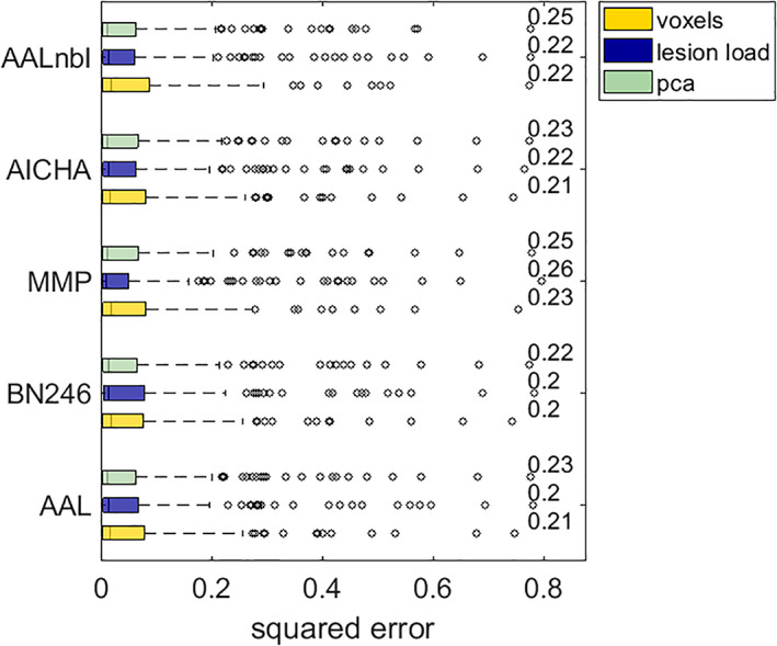
Comparison of feature representations in acute spatial neglect. Boxplots show median and interquartile range of cross‐validation squared errors produced by the model. Whiskers extend to maximally 2.5‐times the interquartile range, and any point beyond that is labelled as an outlier (dots). Numbers indicate each model's R ²

TABLE 3.

Main results

Dataset	Atlas	Chi‐square	p
Neglect	AAL	0.90	.6387
	BN246	0.62	.7332
	MMP	0.80	.6710
	AICHA	0.42	.8091
	AALnbl	0.48	.7855
Hemiparesis	AAL	2.73	.2560
	BN246	2.90	.2343
	MMP	4.47	.1070
	AICHA	6.53	.0382
	AALnbl	6.61	.0367

Note: The table reports results of Friedman tests on prediction residuals between models with the three different lesion representations. We report uncorrected p‐values; no test remained significant after correction for multiple comparisons by the Bonferroni‐Holm procedure. Therefore, no post‐hoc tests were performed.

TABLE 4.

Wilcoxon tests comparing full models and models after feature elimination

	Comparison	Neglect		Hemiparesis
		Z	p	Z	p
AAL	LL full vs. red	1.04	.300	0.32	.750
	PCA full vs. red	1.57	.117	1.06	.289
	LL red vs. PCA red	0.63	.527	1.87	.061
BN246	LL full vs. red	1.67	.095	1.11	.267
	PCA full vs. red	0.67	.500	0.69	.491
	LL red vs. PCA red	0.71	.477	1.97	.049
MMP	LL full vs. red	0.04	.968	0.96	.339
	PCA full vs. red	−0.13	.899	−0.27	.786
	LL red vs. PCA red	0.21	.836	0.72	.472
AICHA	LL full vs. red	0.13	.896	−0.14	.890
	PCA full vs. red	−0.84	.400	0.41	.683
	LL red vs. PCA red	−0.40	.692	1.71	.087
AALnbl	LL full vs. red	0.84	.402	2.03	.042
	PCA full vs. red	1.01	.313	0.13	.900
	LL red vs. PCA red	2.26	.024	0.93	.353

Note: Comparison of full feature sets with the numerically best models after feature elimination, retaining 75, 50 or 25% of the most important features assessed by their permutation importance. ‘red.’ indicates these feature reduced data. Hence, comparisons (a) between full and reduced datasets for all atlases and both lesion load representation and componential representation, and (b) between best feature‐reduced models for all atlases between lesion load representation and componential representation are shown. We report uncorrected p‐values; no test remained significant after correction for multiple comparisons by the Bonferroni‐Holm procedure.

Modelling acute upper limb paresis provided the best cross‐validated model performances overall (Table 2), maxing out at R ² = .316 for a model based on 75% of the most important principal components extracted from voxels contained in the MMP atlas. Overall, model performances for this data set ranged between 0.219 and 0.316, where models based on a principal component representation of the data consistently performed numerically better than models based on patterns of binary voxels or lesion load. However, no significant differences remained after correction for multiple comparisons. Figure 4 gives an overview of the model performances yielded with the three feature representations under each atlas. The numerically least successful models tended to be based on region‐wise lesion load representations. This pattern emerged irrespective of whether we performed backwards elimination of features. Interestingly, before correction for multiple comparisons, there was a significant difference between featurisation strategies for two out of the five parcellations according to the Friedman test (see Table 3). However, after correction for multiple comparisons, no significant results remained and thus we refrained from statistical posthoc comparisons. Again, feature elimination only induced no or, at best, small, non‐significant improvements in model performance (Table 4).

FIGURE 4.

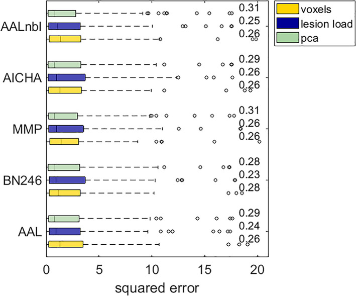
Comparison of feature representations in acute hemiparesis. See the description of Figure 3 for additional information

In summary, we observed that models using a feature representation style that exploits lesion‐anatomical information tended to perform numerically better than those based on region‐wise, parcellation‐dependent information. Furthermore, feature elimination yielded mixed results in terms of model improvement. However, the observed numerical differences did not reach statistical significance.

3.3. Results—comparison of atlases

Across all symptoms, the best CV model performances for lesion load were found for the multimodal parcellation (MMP), which accounted for 25–28% of explained variance. Model performances under the popular morphological AAL atlas tended to be numerically inferior compared to functional parcellations. At the same time, we yielded slight improvements for the predictions of motor scores when we added the white matter tracts from the natbrainlab atlas (see Table 2).

To explore the effect of the five different parcellations on model loss, we conducted a Friedman test on the sample squared errors under models based on lesion load representations of the AAL3, BN246, MMP, AICHA and AALnbl atlases. Results showed that the type of parcellation did not significantly impact model performance neither for neglect (Chi‐square = 8.33, p = .080) nor for hemiparesis (Chi‐square = 1.56, p = .816). For visual descriptive comparison, boxplots of squared errors of lesion load models yielded under different parcellations are shown in Figure S3.

4. DISCUSSION

The current study investigated the suitability of different strategies for feature reduction. We generated and compared structural lesion imaging features based on normalised lesion maps either (i) on a full voxel‐wise level, (ii) transformed into principal components, merging and reducing data following lesion‐anatomical criteria or (iii) transformed into atlas‐based lesion load, merging and reducing data following functional and/or morphological criteria according to the atlases. We found data‐driven principal component‐wise feature representation to provide the numerically best models in almost all conditions. However, we only found minor, non‐significant differences between feature representation strategies, which highlights the general suitability of all feature representations in lesion‐deficit modelling.

While feature representation and feature reduction are central steps in any computer vision algorithm, it has not been a major topic in the field of lesion‐deficit modelling based on structural brain imaging. While all three feature representation strategies that we investigated can be found in previous studies, it often appears as if they have been chosen without elaborated theoretical considerations. Our findings imply that this does not seem to have invalidated these studies. However, these studies might have missed a minor opportunity to potentially maximise model quality by not considering different feature representation strategies.

In many situations in the present study, lesion‐anatomical, componential feature reduction brought forth the numerically best models. Still, numerical differences were relatively minor and not significant. Surprisingly, neither functional, region‐wise feature reduction nor lesion‐anatomical, componential feature reduction allowed significantly better model performance. A voxel‐wise feature representation without any reduction of the high‐dimensional feature space still appears to be a viable option, even though it might be computationally far more demanding. The explanation for this finding might be rooted in the structure of lesion‐deficit data. From a theoretical perspective, there are compelling arguments for both lesion‐anatomical and functional feature reduction. However, both strategies can lead to different and even diametrical solutions (Sperber, 2020). Why this is the case becomes apparent from the granularity of lesions after componential analysis (Zhao et al., 2020). To a large degree, it corresponds to the brain's vasculature underlying the anatomy of stroke, which markedly differs from functional parcellations of the brain (see Zhao et al., 2020). Thus, if we merge voxel‐wise information into two different functional parcels, we might, at the same time, tear apart homogeneous features based on lesion‐anatomical criteria. In other words, two voxels might be frequently damaged together but belong to two separate functional units or, vice versa, might be dissimilar in their lesion status but belong to the same functional module. This also means that, compared to the criteria to subdivide the brain into cortical areas (Eickhoff et al., 2018), stroke imaging adds another potentially conflicting criterion. To conclude, it appears that lesion‐deficit modelling per se suffers from a handicap due to the multifaceted data structure of lesion data.

4.1. Which atlas is best suited to parcellate brain lesions?

For several methodological reasons, a comparison between atlases can only be done with caution and does not allow strong conclusions. First, the overall extent of the atlases differs. An atlas that covers more voxels in the brain can potentially include important brain areas that are highly predictive for a deficit or more irrelevant areas. Second, atlases differ in fine‐graininess by sub‐dividing regions further. Third, popular atlases can be based on either groups or individual subjects, making them differently representative of the average human brain. The Automatic Anatomical Labelling atlas (Rolls et al., 2020), which is often used in lesion‐deficit modelling, is such a single‐subject atlas. More recent brain atlases were often created with large subject groups and multimodal imaging data, including imaging functional and connectomic imaging data. Nonetheless, lesion load representation by the morphological parcellation still allowed comparable lesion‐deficit models, often with only minor differences to multimodal or connectomic parcellations. Thus, the present study does not object to the use of morphological atlases in lesion‐deficit modelling. On the other hand, there are compelling theoretical reasons for the use of state‐of‐the‐art multimodal atlases. Brain parcellations according to morphological criteria do not correspond to the functional organisation of the brain (Eickhoff et al., 2018; Fan et al., 2016; Glasser et al., 2016), while, at the same time, this functional organisation of the brain is often the very topic of our scientific work in cognitive neuroscience. Additionally, the MMP combines information from multimodal neuroimaging from 278 participants and thus allows to account for inter‐subject variability in location and volume of functional modules. A single‐subject atlas like the AAL might not be as generalisable as multi‐subject atlases. Our findings suggest that not modelling performance, but rather such theoretical considerations should be the central factor when choosing a parcellation.

4.2. Implications for lesion‐behaviour mapping

While modelling approaches in post‐stroke outcome prediction and lesion behaviour mapping can be highly similar, there are still pivotal discrepancies between both implied by the purpose of the modelling procedure (Bzdok, Engemann, & Thirion, 2020; Shmueli, 2010). The only purpose of mathematical models in post‐stroke outcome prediction is to make accurate predictions. Hence, explained variance in out‐of‐sample prediction—as the major outcome variable R ² in the present study—is the main criterion to judge a model's success. In lesion‐behaviour mapping, a model's purpose is to identify the neural correlates of behaviour and cognition. This requires some kind of feature‐wise inference, which constitutes a major challenge with very different possible solutions (compare, e.g., Ivanova et al., 2020; Pustina et al., 2018; Zhang et al., 2014). Out‐of‐sample model performance is still of relevance here, but there are more criteria to account for, such as reproducibility of feature weights (Rasmussen, Hansen, Madsen, Churchill, & Strother, 2012). Nonetheless, out‐of‐sample model performance is one of the main criteria for the evaluation of multivariate lesion‐behaviour mapping methods (e.g., Mah, Husain, Rees, & Nachev, 2014; Zhang et al., 2014). Its maximisation with optimal featurisation strategies might improve statistical power in such mapping approaches. An additional challenge arises in lesion‐behaviour modelling as the feature‐wise inferential process puts clear limitations on the way data are modelled. For example, feature elimination is not an option in several approaches that first model data on a whole‐brain level and then access each feature's contribution individually (e.g., Yourganov et al., 2015; Zhang et al., 2014). With respect to the data representation strategies investigated in the present study, voxel‐wise data representation appears to be the most common (e.g., Bates et al., 2003; Pustina et al., 2018; Zhang et al., 2014), yet region‐wise data representation is likewise popular (e.g., Achilles et al., 2017; Smith et al., 2013; Yourganov et al., 2015). The current study suggests that both representations are viable options to create models that capture a decent amount of variance. Hence, region‐wise lesion load models are especially useful in approaches that require a lower‐dimensional representation for computational or mathematical reasons (e.g., Smith et al., 2013; Toba et al., 2017).

But what about componential data after data‐driven feature reduction in lesion‐behaviour mapping? Componential structural lesion imaging data have indeed been used in lesion behaviour mapping (Ivanova et al., 2020; Salvalaggio et al., 2020; Zhao et al., 2020), but they are a rare sight to behold in brain mapping. The main reason for this might be that principal components are difficult to interpret anatomically, which is a crucial final step in the lesion mapping pipeline (de Haan & Karnath, 2018). A single principal component can relate to many widely dispersed voxels to varying degrees. Therefore, a principal component that significantly relates to a deficit cannot be simply assigned to a brain structure. However, principal components can be back‐projected into original voxel‐wise brain space and, under certain conditions, anatomically interpreted.

As we have seen in the present study, the use of componential lesion data only makes a minor, non‐significant difference in out‐of‐sample prediction performance. Still, as discussed above, model performance is only one of several possible criteria in the evaluation of lesion‐behaviour mapping methods (Sperber, 2020; Sperber & Karnath, 2018). A previous methodological validation study assessed several other, more relevant validity criteria in lesion‐behaviour mapping (Ivanova et al., 2020). This study found that multivariate models based on componential lesion data can be beneficial in identifying multi‐regional neural correlates of functions. Importantly, this study also utilised componential feature reduction to make lesion data usable by low‐dimensional multivariate models. This highlights the potential of componential data as an alternative to region‐wise lesion load in mapping methods that are limited in the number of input features (e.g., Smith et al., 2013; Toba et al., 2017). In the current study, we were able to reduce full brain voxel data with over a million features to low‐dimensional datasets of 16–34 components. Such feature reduction can drastically decrease the computational burden of multivariate modelling.

Another argument in favour of using componential data in lesion‐behaviour mapping can be made from a theoretical side. Presenting results of lesion‐behaviour mapping analyses on a voxel level suggests a spatial resolution that simply is not present in the data. With the 1 × 1 × 1 mm³ image resolution utilised in the present study, more than two‐thirds of all voxels can carry information that is perfectly redundant, resulting in much fewer informational ‘unique patches’ than voxels in the dataset (Pustina et al., 2018). Further, both univariate and multivariate lesion mapping are unable to disentangle the contribution of voxels with highly correlated lesion information (Sperber, 2020), and lesion mapping will be unable to differentiate between the role of such voxels. The resolution of lesion behaviour mapping is limited by the informational granularity of lesions (Zhao et al., 2020), which closely follows the vasculature of the brain. Therefore, componential lesion data appears to be a more honest and computationally efficient option in lesion‐behaviour mapping to be considered in future software.

A still open question is if other decompositional algorithms might be better suited to process structural lesion data. We utilised PCA in line with numerous previous studies (e.g., Siegel et al., 2016; Salvalaggio et al., 2020; Zhao et al., 2020). However, other approaches might be better suited to decompose structural lesion data. For example, logistic PCA (Landgraf & Lee, 2020) might be better suited for binary lesion data, and non‐negative matrix factorisation might be a potential approach that refrains from creating negative factors, which do not bear a directly plausible meaning in the context of lesion data.

4.3. How to further improve lesion‐deficit predictions

The variance explained by our models peaked at 32%, a model quality that does not allow clinically relevant predictions. Feature engineering by optimisation of the feature representation is only one possible strategy to optimise lesion‐deficit models. As the current study has shown, this strategy only plays a minor role. However, it is part of a huge arsenal of strategies that have the potential to improve predictions, maybe even up to a critical range where they are applicable in individualised therapy and patient care.

Elimination of irrelevant features might potentially benefit many high‐dimensional modelling algorithms. In the current study, this strategy did not improve model performance significantly. Feature elimination constitutes a difficult challenge in high‐dimensional data. The approach used in our study might not be optimal and could be further optimised. The choice of modelling algorithms might also improve predictions. Support vector regression is only one popular high‐dimensional modelling algorithm out of many. Only a few studies compared different algorithms (e.g., Hope et al., 2018; Rondina et al., 2016), and it might even be the case that no single optimal algorithm exists, but that we require deficit‐specific individual solutions.

The maximisation of lesion‐behaviour model performance is limited by the informational content of the input data. No matter how sophisticated feature engineering and modelling algorithms are, they cannot be better than the information provided by the input data allow. This limits predictions made by lesion‐deficit models based on structural imaging data alone (Sperber, 2020). Many other variables partially explain post‐stroke outcome and a patient's ability to recover, including brain reserve, education, co‐morbidities or intervention (for review, see Price, Hope, & Seghier, 2017). Model performance might suffer from large interpatient variability in time after stroke, as neural plasticity and functional reorganisation might be different in every individual (Price et al., 2017). Hence, the combination of other variables – e.g., demographic data, other imaging data, and non‐imaging biomarkers—will be relevant to obtain highly predictive models. Further, structural lesion imaging is limited in assessing brain pathology, and other imaging modalities assessing connectivity, perfusion or functional activity can—at least for some post‐stroke deficits—complement or replace structural lesion data regarding its informational value (Salvalaggio et al., 2020; Siegel et al., 2016).

4.4. Limitations

In the current study, we encountered several pitfalls that limit model performance and are often encountered in lesion‐behaviour modelling. First, although our sample sizes were relatively large compared to many studies in the field, they were still much smaller than what is often assumed to be optimal for high‐dimensional, multivariate algorithms (see e.g., Mah et al., 2014). Model performance can likely be improved with larger sample sizes. In a previous study, we have shown that voxel‐wise lesion‐behaviour model performance using support vector regression approaches a plateau already with the given sample sizes of ~100 patients (Sperber et al., 2019), albeit small improvements were still present with incremental increases of sample size at this point, and small improvements might well continue even much further. We cannot guarantee that the present findings still hold in much larger samples. Still, we expect that the three investigated featurisation strategies suffered equally from potentially too small samples, and hence allowed valid comparisons. Second, we observed a systematic bias in out‐of‐sample predictions of chronic hemiparesis scores. This partially resulted in models with exceptionally low and uninformative model performances, for which we ultimately removed chronic hemiparesis from the main analysis into the supplementary. Systematic prediction biases were already observed in previous studies (e.g., Loughnan et al., 2019) and can be attributed, to some extent, to the variance and distribution of the target variable. For example, if only a few patients suffer from a deficit, a model might be tuned unintentionally to underestimate the deficit's severity and still perform well in most cases. Hence, the question remains if strategies such as data transformation or the composition of balanced training samples can improve model performance.

From the points discussed in the previous section, some more general limitations of the present study become apparent. We used one single modelling algorithm—support vector regression. Generally, support vector machines and regressions are highly popular in modelling lesion‐behaviour data (e.g., Hope et al., 2018; Mah et al., 2014; Rondina et al., 2016; Rondina et al., 2017; Smith et al., 2013; Zhang et al., 2014). However, Gaussian process regression, regression trees, neural networks and more algorithms are also applicable (e.g., Hope et al., 2013, 2018; Pustina et al., 2018; Rondina et al., 2016). The current study cannot guarantee that the current findings fully apply to the latter algorithms as well. Further, some algorithms such as ridge regression, least absolute shrinkage and selection operator (LASSO) regression and partial least squares regression intrinsically perform dimensionality reduction on underdetermined data. In such a setting, a priori feature reduction might not be as effective as retaining all voxel‐wise features for prediction. In doubt, we suggest including an additional analysis to optimise the feature representation for usage in the designated modelling algorithm. Further, one should be aware that, by using these algorithms on voxel‐wise representations, data are featurised following lesion‐anatomical criteria. Should a better suited functional parcellation for a given deficit exist, such an approach might perform suboptimally. The inclusion of white matter connectivity data was not systematically investigated in the current study. A prominent role of white matter disconnection is assumed for many post‐stroke symptoms (Catani et al., 2012; Griffis, Metcalf, Corbetta, & Shulman, 2019), and numerous complex measures of structural disconnection have been introduced and used in lesion‐(disconnection‐)deficit modelling (e.g., Foulon et al., 2018; Griffis, Metcalf, Corbetta, & Shulman, 2020; Kuceyeski et al., 2016). Notably, these methods are also based on the patients' structural lesion data, which are referred to as healthy controls' connectome data. Thus, these connectome‐based representations also constitute a feature representation of structural lesion data. In the present study, only some of the utilised atlas parcellations included white matter regions. Further, consider a white matter tract whose cross‐section is lesioned, causing complete disconnection. In this case, lesion load is small relative to the whole volume, underestimating the severity of the disconnection. Where the two measures of lesion load and tract disconnection diverge, analyses based on lesion load can mask a real relationship between tract damage and the severity of some deficit of interest (Hope, Seghier, Prejawa, Leff, & Price, 2016). We currently view the optimisation of feature representation strategies for structural disconnection as another major challenge, which goes beyond the scope of the current study and requires separate extensive empirical studies.

5. CONCLUSIONS

Feature representation strategies have the potential to improve lesion‐deficit modelling. Yet, it is only one of many methodological strategies to improve models, with only minor benefits if applied alone. The present study found data‐driven component‐wise feature representation to provide the numerically best performing models in most situations, while voxel‐based and atlas‐based lesion load representation was found to be non‐significantly inferior. Thus, if methodological or theoretical considerations suggest a lesion‐load data representation, such can be used. We suggest that if a study intends to maximise a model's predictive power, feature representation strategies are taken into consideration and compared.

CONFLICT OF INTEREST

The authors declare no conflict of interest.

Supporting information

Appendix S1: Supporting information

Figure S1—Overlap topographies of normalised lesion maps

Figure S2—Example scree graph after principal component analysis.

Figure S3—Boxplots of lesion load model squared errors per atlas.

Figure S4—Correlation plot of predicted and measured scores of chronic limb paresis.

Kasties, V. , Karnath, H.‐O. , & Sperber, C. (2021). Strategies for feature extraction from structural brain imaging in lesion‐deficit modelling. Human Brain Mapping, 42(16), 5409–5422. 10.1002/hbm.25629

DATA AVAILABILITY STATEMENT

The data that support the findings of this study are openly available in Mendeley Data at http://dx.doi.org/10.17632/34rwd5vb2h.2. Original clinical data are not publicly available due to privacy and ethical restrictions.

REFERENCES

- Achilles, E. I. S. , Weiss, P. H. , Fink, G. R. , Binder, E. , Price, C. J. , & Hope, T. M. H. (2017). Using multi‐level Bayesian lesion‐symptom mapping to probe the body‐part‐specificity of gesture imitation skills. NeuroImage, 161, 94–103. [DOI] [PMC free article] [PubMed] [Google Scholar]
- Arlot, S. , & Celisse, A. (2010). A survey of cross‐validation procedures for model selection. Statistics Surveys, 4, 40–79. [Google Scholar]
- Bates, E. , Wilson, S. M. , Saygin, A. P. , Dick, F. , Sereno, M. I. , Knight, R. T. , & Dronkers, N. F. (2003). Voxel‐based lesion‐symptom mapping. Nature Neuroscience, 6, 448–450. [DOI] [PubMed] [Google Scholar]
- Breiman, L. (2001). Random forests. Machine Learning, 45, 5–32. [Google Scholar]
- Bzdok, D. , Engemann, D. , & Thirion, B. (2020). Inference and Prediction Diverge in Biomedicine. Patterns, 1, 100119. 10.1016/j.patter.2020.100119 [DOI] [PMC free article] [PubMed] [Google Scholar]
- Catani, M. , Dell'Acqua, F. , Bizzi, A. , Forkel, S. J. , Williams, S. C. , Simmons, A. , … Thiebaut de Schotten, M. (2012). Beyond cortical localization in clinico‐anatomical correlation. Cortex, 48, 1262–1287. 10.1016/j.cortex.2012.07.001 [DOI] [PubMed] [Google Scholar]
- Catani, M. , & Thiebaut de Schotten, M. (2008). A diffusion tensor imaging tractography atlas for virtual in vivo dissections. Cortex, 44, 1105–1132. [DOI] [PubMed] [Google Scholar]
- Chang, C. , & Lin, C. (2011). LIBSVM. ACM Transactions on Intelligent Systems and Technology, 2, 1–27. [Google Scholar]
- de Haan, B. , Clas, P. , Juenger, H. , Wilke, M. , & Karnath, H. O. (2015). Fast semi‐automated lesion demarcation in stroke. NeuroImage: Clinical, 9, 69–74. 10.1016/j.nicl.2015.06.013 [DOI] [PMC free article] [PubMed] [Google Scholar]
- de Haan, B. , & Karnath, H.‐O. (2018). A hitchhiker' s guide to lesion‐behaviour mapping. Neuropsychologia, 115, 5–16. [DOI] [PubMed] [Google Scholar]
- Eickhoff, S. B. , Constable, R. T. , & Yeo, B. T. T. (2018). Topographic organization of the cerebral cortex and brain cartography. NeuroImage, 170, 332–347. [DOI] [PMC free article] [PubMed] [Google Scholar]
- Fan, L. , Li, H. , Zhuo, J. , Zhang, Y. , Wang, J. , Chen, L. , … Jiang, T. (2016). The Human Brainnetome Atlas: A New Brain Atlas Based on Connectional Architecture. Cerebral Cortex, 26, 3508–3526. [DOI] [PMC free article] [PubMed] [Google Scholar]
- Feng, W. , Wang, J. , Chhatbar, P. Y. , Doughty, C. , Landsittel, D. , Lioutas, V.‐A. , … Schlaug, G. (2015). Corticospinal tract lesion load: An imaging biomarker for stroke motor outcomes. Annals of Neurology, 78, 860–870. [DOI] [PMC free article] [PubMed] [Google Scholar]
- Fisher, A. , Rudin, C. , Dominici, F. (2018). Model class reliance: Variable importance measures for any machine learning model class, from the “rashomon” perspective. arXiv preprint arXiv:1801.01489, 68.
- Foulon, C. , Cerliani, L. , Kinkingnéhun, S. , Levy, R. , Rosso, C. , Urbanski, M. , … Thiebaut de Schotten, M. (2018). Advanced lesion symptom mapping analyses and implementation as BCBtoolkit. Gigascience, 7, 1–17 http://biorxiv.org/content/early/2017/05/02/133314 [DOI] [PMC free article] [PubMed] [Google Scholar]
- Gauthier, L. , Dehaut, F. , & Joanette, Y. (1989). The Bells Test: A quantitative and qualitative test for visual neglect. International Journal of Clinical Neuropsychology, 11(2), 49–54. [Google Scholar]
- Glasser, M. F. , Coalson, T. S. , Robinson, E. C. , Hacker, C. D. , Harwell, J. , Yacoub, E. , … Van Essen, D. C. (2016). A multimodal parcellation of human cerebral cortex. Nature, 536, 171–178. [DOI] [PMC free article] [PubMed] [Google Scholar]
- Griffis, J. C. , Metcalf, N. V. , Corbetta, M. , & Shulman, G. L. (2019). Structural disconnections explain brain network dysfunction after stroke. Cell Reports, 28, 2527–2540. 10.1016/j.celrep.2019.07.100 [DOI] [PMC free article] [PubMed] [Google Scholar]
- Griffis, J. C. , Metcalf, N. V. , Corbetta, M. , Shulman, G. L. (2020). Lesion quantification toolkit: A MATLAB software tool for estimating grey matter damage and white matter disconnections in patients with focal brain lesions. bioRxiv 2020.07.28.225771. 10.1101/2020.07.28.225771 [DOI] [PMC free article] [PubMed]
- Hillis, A. E. , Beh, Y. Y. , Sebastian, R. , Breining, B. , Tippett, D. C. , Wright, A. , … Fridriksson, J. (2018). Predicting recovery in acute poststroke aphasia. Annals of Neurology, 83, 612–622. [DOI] [PMC free article] [PubMed] [Google Scholar]
- Holm, S. (1979). A simple sequentially rejective multiple test procedure. Scandinavian Journal of Statistics, 6, 65–70. [Google Scholar]
- Hope, T. M. H. , Leff, A. P. , & Price, C. J. (2018). Predicting language outcomes after stroke: Is structural disconnection a useful predictor? NeuroImage: Clinical, 19, 22–29. [DOI] [PMC free article] [PubMed] [Google Scholar]
- Hope, T. M. H. , Seghier, M. L. , Leff, A. P. , & Price, C. J. (2013). Predicting outcome and recovery after stroke with lesions extracted from MRI images. NeuroImage Clin, 2, 424–433. 10.1016/j.nicl.2013.03.005 [DOI] [PMC free article] [PubMed] [Google Scholar]
- Hope, T. M. H. , Seghier, M. L. , Prejawa, S. , Leff, A. P. , & Price, C. J. (2016). Distinguishing the effect of lesion load from tract disconnection in the arcuate and uncinate fasciculi. NeuroImage, 125, 1169–1173. 10.1016/j.neuroimage.2015.09.025 [DOI] [PMC free article] [PubMed] [Google Scholar]
- Horn, J. L. (1965). A rationale and test for the number of factors in factor analysis. Psychometrika, 30, 179–185. 10.1007/BF02289447 [DOI] [PubMed] [Google Scholar]
- Hsu, C. W. , Chang, C. C. , Lin, C. J. (2003). A practical guide to support vector classification Retrieved from https://www.csie.ntu.edu.tw/~cjlin/papers/guide/guide.pdf.
- Hua, K. , Zhang, J. , Wakana, S. , Jiang, H. , Li, X. , Reich, D. S. , … Mori, S. (2008). Tract probability maps in stereotaxic spaces: Analyses of white matter anatomy and tract‐specific quantification. NeuroImage, 39, 336–347. [DOI] [PMC free article] [PubMed] [Google Scholar]
- Ivanova, M. V. , Herron, T. J. , Dronkers, N. F. , & Baldo, J. V. (2020). An empirical comparison of univariate versus multivariate methods for the analysis of brain–behavior mapping. Human Brain Mapping, 42, 1070–1101. 10.1002/hbm.25278 [DOI] [PMC free article] [PubMed] [Google Scholar]
- James, G. , Witten, D. , Hastie, T. , & Tibshirani, R. (2013). An introduction to statistical learning (Vol. 112). New York, NY: Springer. [Google Scholar]
- Joliot, M. , Jobard, G. , Naveau, M. , Delcroix, N. , Petit, L. , Zago, L. , … Tzourio‐Mazoyer, N. (2015). AICHA: An atlas of intrinsic connectivity of homotopic areas. Journal of Neuroscience Methods, 254, 46–59. 10.1016/j.jneumeth.2015.07.013 [DOI] [PubMed] [Google Scholar]
- Kuceyeski, A. , Navi, B. B. , Kamel, H. , Raj, A. , Relkin, N. , Toglia, J. , … O'Dell, M. (2016). Structural connectome disruption at baseline predicts 6‐months post‐stroke outcome. Human Brain Mapping, 2601, 2587–2601. [DOI] [PMC free article] [PubMed] [Google Scholar]
- Landgraf, A. J. , & Lee, Y. (2020). Dimensionality reduction for binary data through the projection of natural parameters. Journal of Multivariate Analysis, 180, 104668. 10.1016/j.jmva.2020.104668 [DOI] [Google Scholar]
- Loughnan, R. , Lorca‐Puls, D. L. , Gajardo‐Vidal, A. , Espejo‐Videla, V. , Gillebert, C. R. , Mantini, D. , … Hope, T. M. H. (2019). Generalizing post‐stroke prognoses from research data to clinical data. NeuroImage: Clinical, 24, 102005. 10.1016/j.nicl.2019.102005 [DOI] [PMC free article] [PubMed] [Google Scholar]
- Mah, Y.‐H. , Husain, M. , Rees, G. , & Nachev, P. (2014). Human brain lesion‐deficit inference remapped. Brain, 137, 2522–2531. [DOI] [PMC free article] [PubMed] [Google Scholar]
- Price, C. J. , Hope, T. M. , & Seghier, M. L. (2017). Ten problems and solutions when predicting individual outcome from lesion site after stroke. NeuroImage, 145, 200–208. 10.1016/j.neuroimage.2016.08.006 [DOI] [PMC free article] [PubMed] [Google Scholar]
- Pustina, D. , Avants, B. , Faseyitan, O. K. , Medaglia, J. D. , & Coslett, H. B. (2018). Improved accuracy of lesion to symptom mapping with multivariate sparse canonical correlations. Neuropsychologia, 115, 154–166. 10.1016/j.neuropsychologia.2017.08.027 [DOI] [PubMed] [Google Scholar]
- Rasmussen, P. M. , Hansen, L. K. , Madsen, K. H. , Churchill, N. W. , & Strother, S. C. (2012). Model sparsity and brain pattern interpretation of classification models in neuroimaging. Pattern Recognition, 45, 2085–2100. 10.1016/j.patcog.2011.09.011 [DOI] [Google Scholar]
- Rolls, E. T. , Huang, C.‐C. , Lin, C.‐P. , Feng, J. , & Joliot, M. (2020). Automated anatomical labelling atlas 3. NeuroImage, 206, 116189. 10.1016/j.neuroimage.2019.116189 [DOI] [PubMed] [Google Scholar]
- Rondina, J. M. , Filippone, M. , Girolami, M. , & Ward, N. S. (2016). Decoding post‐stroke motor function from structural brain imaging. NeuroImage: Clinical, 12, 372–380. 10.1016/j.nicl.2016.07.014 [DOI] [PMC free article] [PubMed] [Google Scholar]
- Rondina, J. M. , Park, C. , & Ward, N. S. (2017). Brain regions important for recovery after severe post‐stroke upper limb paresis. Journal of Neurology, Neurosurgery, and Psychiatry, 88, 737–743. 10.1136/jnnp-2016-315030 [DOI] [PMC free article] [PubMed] [Google Scholar]
- Rorden, C. , Bonilha, L. , Fridriksson, J. , Bender, B. , & Karnath, H. O. (2012). Age‐specific CT and MRI templates for spatial normalization. NeuroImage, 61, 957–965. [DOI] [PMC free article] [PubMed] [Google Scholar]
- Rorden, C. , & Karnath, H. O. (2004). Using human brain lesions to infer function: A relic from a past era in the fMRI age? Nature Reviews. Neuroscience, 5, 812–819. [DOI] [PubMed] [Google Scholar]
- Rorden, C. , & Karnath, H. O. (2010). A simple measure of neglect severity. Neuropsychologia, 48, 2758–2763. 10.1016/j.neuropsychologia.2010.04.018 [DOI] [PMC free article] [PubMed] [Google Scholar]
- Salvalaggio, A. , De Filippo De Grazia, M. , Zorzi, M. , Thiebaut de Schotten, M. , & Corbetta, M. (2020). Post‐stroke deficit prediction from lesion and indirect structural and functional disconnection. Brain, 143, 2173–2188. [DOI] [PMC free article] [PubMed] [Google Scholar]
- Shmueli, G. (2010). To Explain or to Predict? Statistical Science, 25, 289–310. 10.1214/10-STS330 [DOI] [Google Scholar]
- Siegel, J. S. , Ramsey, L. E. , Snyder, A. Z. , Metcalf, N. V. , Chacko, R. V. , Weinberger, K. , … Corbetta, M. (2016). Disruptions of network connectivity predict impairment in multiple behavioral domains after stroke. Proceedings of the National Academy of Sciences, 113, E4367–E4376. 10.1073/pnas.1521083113 [DOI] [PMC free article] [PubMed] [Google Scholar]
- Smith, D. V. , Clithero, J. A. , Rorden, C. , & Karnath, H.‐O. (2013). Decoding the anatomical network of spatial attention. Proceedings of the National Academy of Sciences, 110, 1518–1523. [DOI] [PMC free article] [PubMed] [Google Scholar]
- Smola, A. J. , & Schölkopf, B. (2004). A tutorial on support vector regression. Statistics and Computing, 14, 199–222. [Google Scholar]
- Sperber, C. (2020). Rethinking causality and data complexity in brain lesion‐behaviour inference and its implications for lesion‐behaviour modelling. Cortex, 126, 49–62. 10.1016/j.cortex.2020.01.004 [DOI] [PubMed] [Google Scholar]
- Sperber, C. , & Karnath, H.‐O. (2017). Impact of correction factors in human brain lesion‐behavior inference. Human Brain Mapping, 38, 1692–1701. 10.1002/hbm.23490 [DOI] [PMC free article] [PubMed] [Google Scholar]
- Sperber, C. , & Karnath, H.‐O. (2018). On the validity of lesion‐behaviour mapping methods. Neuropsychologia, 115, 17–24. 10.1016/j.neuropsychologia.2017.07.035 [DOI] [PubMed] [Google Scholar]
- Sperber, C. , Wiesen, D. , & Karnath, H. O. (2019). An empirical evaluation of multivariate lesion behaviour mapping using support vector regression. Human Brain Mapping, 40, 1381–1390. 10.1002/hbm.24476 [DOI] [PMC free article] [PubMed] [Google Scholar]
- Toba, M. N. , Zavaglia, M. , Rastelli, F. , Valabrégue, R. , Pradat‐Diehl, P. , Valero‐Cabré, A. , & Hilgetag, C. C. (2017). Game theoretical mapping of causal interactions underlying visuo‐spatial attention in the human brain based on stroke lesions. Human Brain Mapping, 38, 3454–3471. 10.1002/hbm.23601 [DOI] [PMC free article] [PubMed] [Google Scholar]
- Varoquaux, G. , Raamana, P. R. , Engemann, D. A. , Hoyos‐Idrobo, A. , Schwartz, Y. , & Thirion, B. (2017). Assessing and tuning brain decoders: Cross‐validation, caveats, and guidelines. NeuroImage, 145, 166–179. 10.1016/j.neuroimage.2016.10.038 [DOI] [PubMed] [Google Scholar]
- Weintraub, S. , & Mesulam, M. (1985). Mental state assessment of young and elderly adults in behavioral neurology. In Mesulam M. (Ed.), Principles of behavioural neurology. Philadelphia, PA: F. A. Davis Company. [Google Scholar]
- Wiesen, D. , Sperber, C. , Yourganov, G. , Rorden, C. , & Karnath, H. O. (2019). Using machine learning‐based lesion behavior mapping to identify anatomical networks of cognitive dysfunction: Spatial neglect and attention. NeuroImage, 201, 116000. 10.1101/556753 [DOI] [PMC free article] [PubMed] [Google Scholar]
- Xu, T. , Rolf Jäger, H. , Husain, M. , Rees, G. , & Nachev, P. (2018). High‐dimensional therapeutic inference in the focally damaged human brain. Brain, 141, 48–54. [DOI] [PMC free article] [PubMed] [Google Scholar]
- Yourganov, G. , Smith, K. G. , Fridriksson, J. , & Rorden, C. (2015). Predicting aphasia type from brain damage measured with structural MRI. Cortex, 73, 203–215. [DOI] [PMC free article] [PubMed] [Google Scholar]
- Zhang, Y. , Kimberg, D. Y. , Coslett, H. B. , Schwartz, M. F. , & Wang, Z. (2014). Multivariate lesion‐symptom mapping using support vector regression. Human Brain Mapping, 35, 5861–5876. [DOI] [PMC free article] [PubMed] [Google Scholar]
- Zhao, Y. , Halai, A. D. , & Lambon Ralph, M. A. (2020). Evaluating the granularity and statistical structure of lesions and behaviour in post‐stroke aphasia. Brain Communications, 2, 1–14. [DOI] [PMC free article] [PubMed] [Google Scholar]
Associated Data
This section collects any data citations, data availability statements, or supplementary materials included in this article.
Supplementary Materials