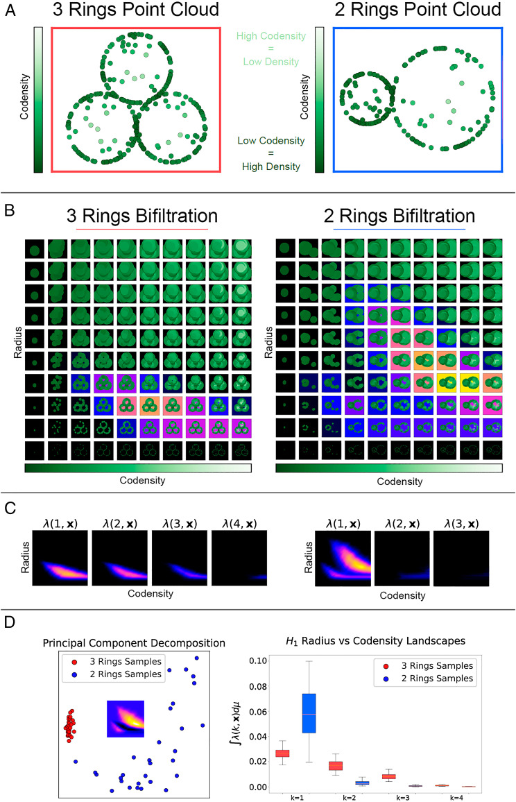
Fig. 2.

We illustrate the features of point cloud data which may be extracted by MPH and associated landscapes (MPH landscapes). (A) Point clouds from rings of different radii, together with measurement noise, to demonstrate that MPH landscapes can detect the size and number of loops in the presence of noise. Eighty points are uniformly sampled from each ring, and 20 points are sampled from the area enclosed by each ring. (B) Illustrations of the radius-codensity bifiltrations associated with the example point clouds. Increasing the radius parameter increases the radius of the balls centered at the points of the point cloud. The codensity parameter first admits points from dense regions of the point cloud (dark green) and then includes points from the sparser regions (light green). We highlight the parameter values for which loops are formed in the bifiltration; the strongest signal of a loop is shown in yellow. (C) The MPH landscapes for the bifiltrations highlight the regions of the parameter space for which loops are detected. For the 3 Rings point cloud we detect a signal above small radius parameters in $\lambda \left(1,\overrightarrow{x}\right),\lambda \left(2,\overrightarrow{x}\right)$ and $\lambda \left(3,\overrightarrow{x}\right)$ but not $\lambda \left(4,\overrightarrow{x}\right)$. These signals correspond to the three small loops of the same scale in the point cloud. For the 2 Rings point cloud we detect a signal above large radius and large codensity parameters and a signal for small radius and small codensity parameters in $\lambda \left(1,\overrightarrow{x}\right)$. These signals correspond to the large radius sparsely sampled loop and the small radius densely sampled loop respectively. (D) Taking 30 samples of each of the point clouds and treating the output persistence landscapes as high dimensional vectors. PCA of the vectors $\lambda \left(1,\overrightarrow{x}\right)$ identifies that the principal difference between the two types of point clouds is the presence of a large radius loop. Taking the norm of the landscape vectors outputs a real value. We plot the distributions of the norms $\Vert \lambda \left(k,\overrightarrow{x}\right)\Vert ,k=\mathrm{1,2,3,4}$ for the two point clouds. These distributions identify a large loop in the 2 Rings point clouds and three loops in the 3 Rings point clouds.