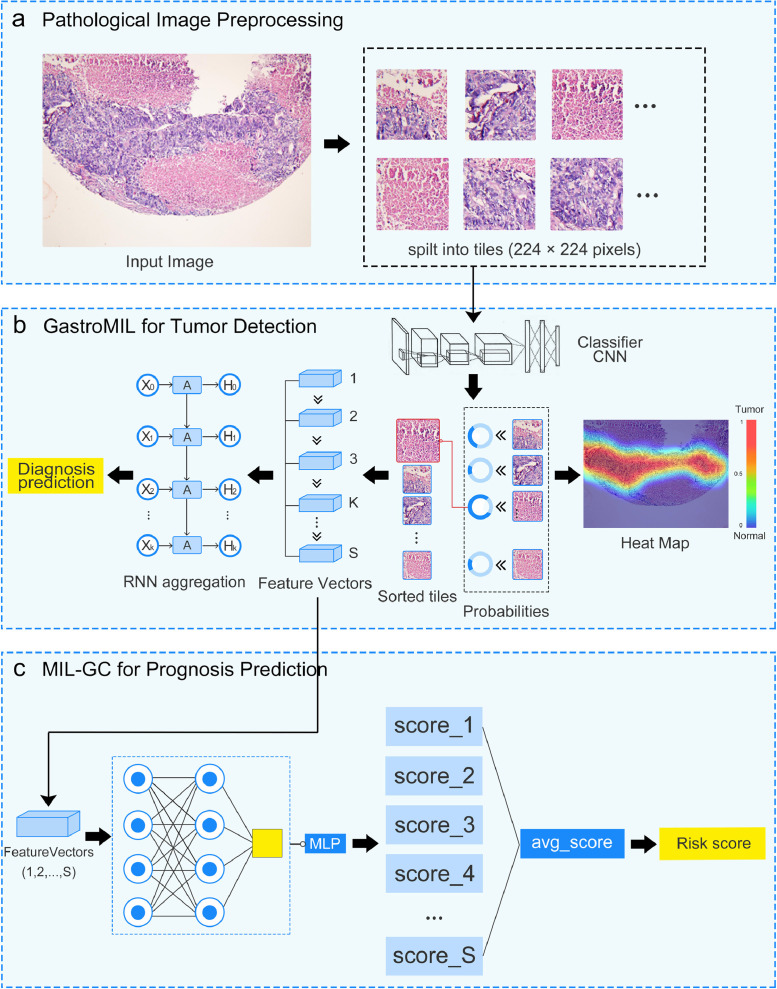
Fig. 1.

Flow chart of the developed models. The framework of GastroMIL is shown in a-b, and that of MIL-GC is shown in a-c. Pathological images are input and tiles with 224 × 224 pixels of each image are generated (a). Through CNN classifier of the MIL model, the probability of these tiles being malignant is output. Heat map visualizes ROIs identified by the model. Feature vectors with dimension 608 of the most suspicious tiles are extracted. Feature vectors of the K most suspicious tiles are input to the second layer of MIL and aggregated by RNN, and then the final diagnosis prediction of the input image is generated. In this study we took K as 32 (b). Feature vectors of the most S suspicious tiles are input to the prognosis model (in this study S = 128). In the MIL-GC model, each feature vector yields a probability value through a MLP algorithm. Probability values of the 128 most suspicious tiles of the input picture were merged to generate an average value as the output risk score (c). CNN, convolutional neural network; RNN, recurrent neural network; MIL, multiple instance learning; MLP, multilayer perceptron; ROI, region of interest.