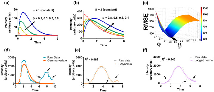
Figure 1.

Illustration of curve fitting and optimization process. (a–d) GV curve fitting by optimizing unknown parameters, (a) α and (b) β. Change in β changes the magnitude whereas variation in α changes the shape of the curve (rate of decay), (c) selection of α and β based on least root mean square error (RMSE) (arrow), (d) raw data, and final reference curve based on GV function. Reference curves based on (e) polynomial, and (f) lagged normal curve-fit functions. Recirculation and random intensity variations (shown by arrows in raw data) are absent in the fitted curves.