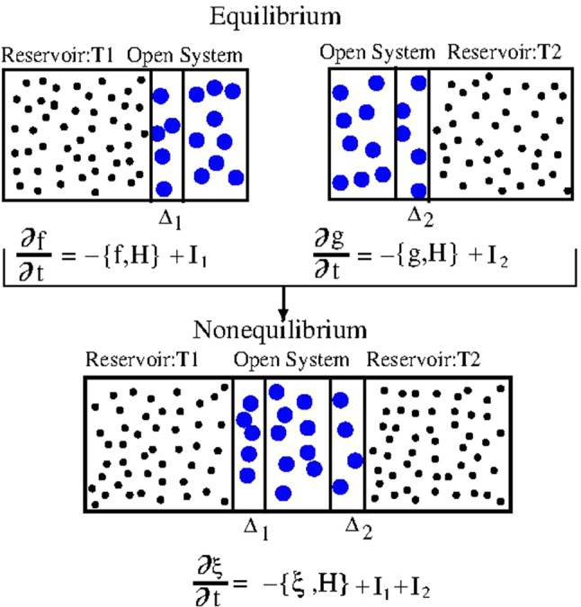
Fig. 17.

Pictorial illustration of the application of the linear action of the reservoirs in AdResS for the case of a thermal gradient. The system is first considered at equilibrium, at the thermodynamic condition of each reservoir, separately. Two separate simulations determine in AdResS $F_{\text{th}}^1(x)$ and $F_{\text{th}}^2(x)$. The open system is then put in contact with two different reservoirs; the mathematical models prescribe the linear action of the reservoirs: $I^{(1)}+I^{(2)}$. The linear action of the mathematical models in AdResS corresponds to the action of $F_{\text{th}}^{(1)}(x)$ and an external thermostat that keeps the temperature at $T_1$ in the region ${\Delta }_1+{\text{TR}}_1$ and to the action of $F_{\text{th}}^{(2)}(x)$ and an external thermostat that keeps the temperature at $T_2$ in ${\Delta }_2+{\text{TR}}_2$, that is: $I^{(1)}=F_{\text{th}}^{(1)}(x)+Thermostat\left(T_1\right)$ and $I^{(2)}=F_{\text{th}}^{(2)}(x)+Thermostat\left(T_2\right)$ so that $I^{(1)}+I^{(2)}=F_{\text{th}}^{(1)}(x)+Thermostat\left(T_1\right)+F_{\text{th}}^{(2)}(x)+Thermostat\left(T_2\right)$