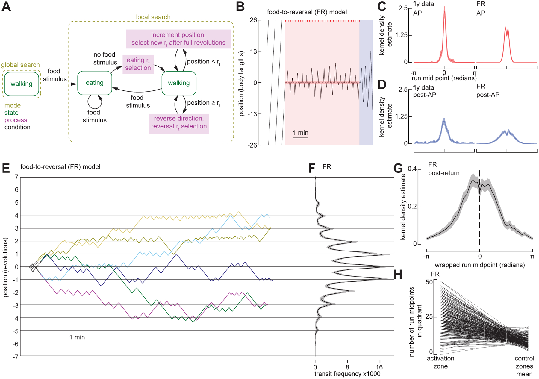
Figure 3. An agent-based model using iterative odometric integration recapitulates Drosophila local search around a single fictive food site.

(A) Schematic of the state-transition diagram for an agent-based model. Arrows indicate transitions—governed by conditions—between search modes, behavioral states, and computational processes. For detailed state transition diagrams, including that of the simulated environment, see Figure S3.

(B) Example trajectory of FR model simulation in a circular arena with a 52-body length circumference, showing baseline, AP, and post-AP. Plotting conventions as in Figure 1B.

(C) Normalized kernel density estimate (KDE) of the run midpoint in during AP for flies (left, N = 22 flies) and FR model (right, N = 300). Data for the fly is re-plotted from Figure 1M.

(D) Normalized kernel density estimate (KDE) of the run midpoint in during post-AP for flies (left, N = 22 flies) and FR model (right, N = 300). Data for the fly is re-plotted from Figure 1M.

(E) Six representative example trajectories of FR model simulation in a small circular arena with a 26-body length circumference (same as experiments in Figure 2). Plotting conventions as in Figure 2B.

(F) Mean transit distribution for FR simulations in small arena. (N = 300). Plotting conventions as in Figure 2E.

(G) Normalized kernel density estimate (KDE) of the wrapped run midpoint in the post-return period for FR simulations in small arena. (N = 300). Plotting conventions as in Figure 2F.

(H) Number of run midpoints in the food quadrant compared to the other three quadrants during post-return trajectories for FR simulations in small arena. (N = 300). Each line shows the values for a single simulation, where data from all three control quadrants were averaged together.