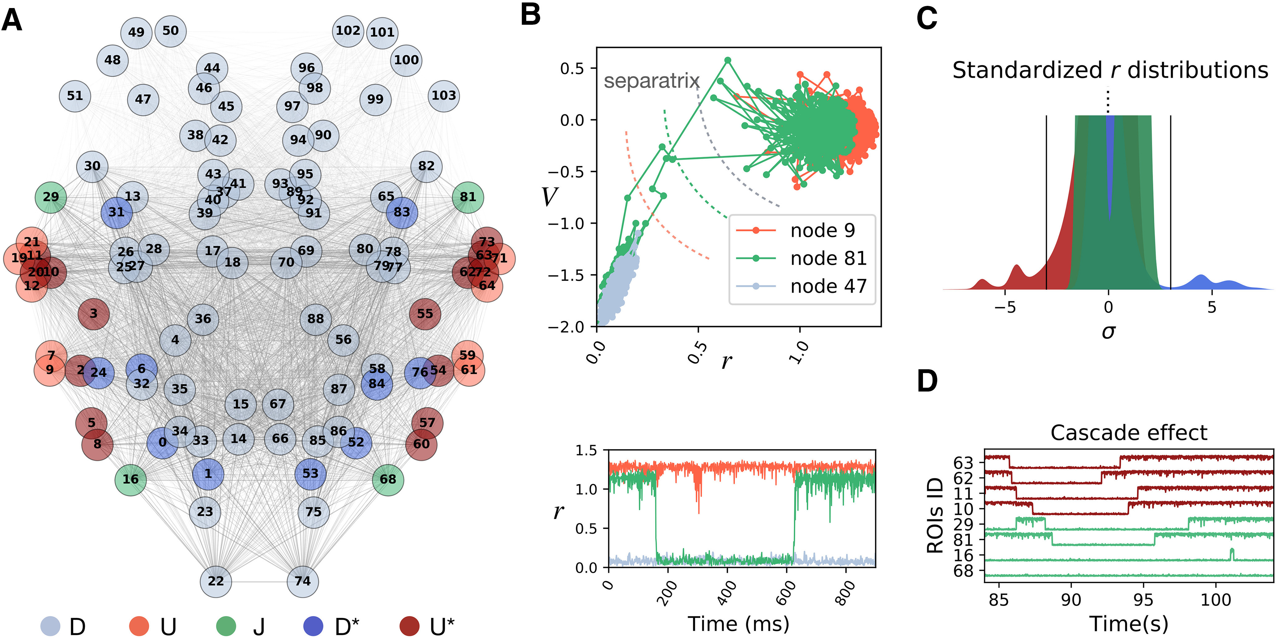
Figure 4.

Mechanisms of cascade generation in the synthetic model. A, Different regions have a different fate depending on their location in the connectome. We classified the regions in five classes (D, U, J, D*, U*) according to their activity. B, Example exploration of the projected 2D phase space (top) and firing rates activity (bottom) of the “up-U” (light red), “down-D” (light blue), and “jumping-J” (green) regions. C, Distribution of the standardized firing rates in different classes. Class (J) regions have two modes but never cross the ±3 σ threshold (black lines). Class (U*) (dark blue) and class (D*) (dark red) regions dwell most of the time in the up and down states, respectively. Only in important rare occasions the *-regions cross the threshold to jump on the other side, substantially deviating from their baseline activity. The leading role of the *-regions as compared with the other classes is shown using PCA in Extended Data Figure 4-1A,B. D, Example of a cascade: when the (U*) node 63 jumps into the down state, it first drags down the node 62 (with which it shares the strongest structural link in the network). After them, other strongly connected nodes follow the trend.