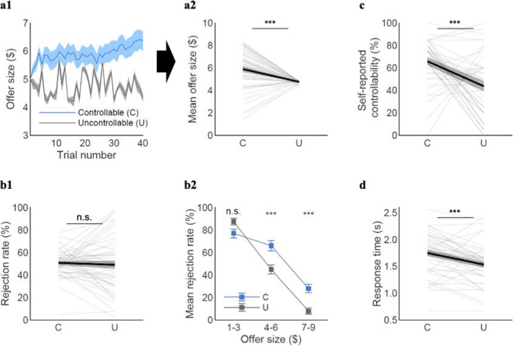
Figure 2. Model-agnostic behavioral results.

(a1) Participants raised the offers along the trials when they had control (Controllable), compared to when they had no control (Uncontrollable). (a2) The mean offer size was higher for the Controllable (C) than Uncontrollable (U) condition (mean_C=5.9, mean_U=4.8, t(47.45)=4.33, p<0.001). (b1) Overall rejection rates were not different between the two conditions (mean_C=50.8%, mean_U=49.1%, t(67.87)=0.43, p=0.67). (b2) However, participants were more likely to reject middle and high offers when they had control (low ($1–3): mean_C=77%, mean_U=87%, t(22)=–1.35, p=0.19; middle ($4–6): mean_C=66%, mean_U=45%, t(47)=5.41, p<0.001; high ($7–9): mean_C=28%, mean_U=8%, t(72.50)=4.00, p<0.001). Each offer bin for the Controllable in (b2) represents 23, 48, and 41 participants who were proposed the corresponding offers at least once, whereas each bin for the Uncontrollable represents all 48 participants. The t-test for each bin was conducted for those who had the corresponding offers for both conditions. (c) The self-reported controllability ratings were higher for the Controllable than Uncontrollable condition (mean_C=65.9, mean_U=43.7, t(74.55)=4.10, p<0.001; eight participants were excluded due to missing data). (d) Response times were longer for the Controllable than the Uncontrollable condition (mean_C=1.75±0.38, mean_U=1.53±0.38; paired t-test t(47)=4.34, p<0.001), suggesting that participants were likely to engage more deliberation during decision-making in the Controllable condition. A paired t-test was used for the rejection rates for low and middle offers and the self-reported controllability ratings. The t-statistics for the mean offer size, overall rejection rate, rejection rate for high offers, and self-reported controllability are from two-sample t-tests assuming unequal variance using Satterthwaite’s approximation according to the results of the F-tests for equal variance. Error bars and shades represent SEM; ***p<0.001; n.s. indicates not significant. For (a2, b1, c, d), each line represents a participant and each bold line represents the mean.

Figure 2—figure supplement 1. Behavioral results of a non-social controllability task.

To investigate whether our results are specific to the social domain, we ran another batch of the task in which 27 out of the 48 original participants were re-contacted with a 14- to 24-month temporal gap and played the same game with the instruction of ‘playing with computer’ instead of ‘playing with virtual human partners.’ Overall, we found choice patterns (a–f) similar to those in the social task, while the subjective states (i.e., self-reported controllability) (g) and the impact of the norm prediction error on the emotion ratings (Supplementary file 1) differed from the social task. (a) Similar to the results of the social task, offers (mean_C=6.0, mean_U=4.7, t(26.23)=3.03, p<0.01) were higher for the Controllable than the Uncontrollable. (b) Overall rejection rates (mean_C=55.9%, mean_U=58.1%, t(40.76)=–0.33, p=0.74) or (c) any of the binned rejection rates were not significantly different between the two conditions (paired t-test; low ($1–3): mean_C=76%, mean_U=81%, t(12)=1.54, p=0.15; middle ($4–6): mean_C=64%, mean_U=56%, t(26)=1.74, p=0.09; high ($7–9): mean_C=39%, mean_U=29%, t(19)=0.80, p=0.44). (d, e) The DIC scores showed a similar pattern to the social task, with the elbow point at the 2-step FT model for both conditions. Paired t-tests confirmed that the 2-step model’s DIC scores were significantly lower than the 0-step model (Controllable: t(26)=–3.16, p<0.01; Uncontrollable: t(26)=–2.38, p<0.05) and the 1-step model (Controllable: t(26)=–3.02, p<0.01; Uncontrollable: t(26)=–2.31, p<0.05), whereas the DIC scores were not significantly different between the 2-step model and the 3-step model (Controllable: t(26)=–1.23, p=0.23; Uncontrollable: t(26)=0.20, p=0.84) or the 4-step model (Controllable: t(26)=0.68, p=0.50; Uncontrollable: t(26)=–0.13, p=0.90). (f) Expected influence was significantly higher for the Controllable than the Uncontrollable condition (mean_C=1.31, mean_U=0.75, t(26)=2.54, p<0.05). (g) In contrast to the social task, self-reported controllability was not different between the two conditions when individuals played the game with a computer (mean_C=62.7, mean_U=56.9, t(25)=0.78, p=0.44). (h) To unpack the norm prediction error×social interaction effect in Supplementary file 1a, we used the regression coefficients from the original mixed-effect regression (‘emotion rating~ offer+norm prediction error+condition+task+task*(offer+norm prediction error+condition)+(1+offer+norm prediction error | subject)’) and calculated the residual, which should be explained by the differential impact of nPE between social and non-social tasks. Correlation coefficients between the residuals and nPE were plotted for each task condition (mean_Social=0.151, mean_Non-social=0.005; SD_Social=0.023, SD_Non-social=0.025). Note that the non-social task was coded as the reference group (0 for the group identifier) in our original regression. This result indicates that the impact of nPE was stronger in the social than in the non-social Computer task. Bars represent the mean of the coefficients and error bars represent the standard deviation. (i) To unpack the Controllable×social task interaction effect in Supplementary file 1a, similar to (h), we used the coefficients from the original mixed-effect regression (‘emotion rating~ offer+norm prediction error+condition+task+task*(offer+norm prediction error+condition)+(1+offer+norm prediction error | subject)’) and calculated the residual by each condition and task as shown in the figure (mean_Social(C)=–5.00, mean_Social(U)=–0.58, mean_Computer(C)=0.63, mean _Computer(U)=0.00; SEM_Social(C)=0.46, SEM_Social(U)=0.43, SEM_Computer(C)=0.72, SEM_Computer(U)=0.77). Bars represent the mean of the coefficients and error bars represent SEM. Note that the non-social task and the Uncontrollable condition were coded as the reference group (0 for the group identifiers) in the regression. These results show that the emotion ratings were lower in the Controllable social context compared to the non-social as well as the Uncontrollable social context. We speculate that exerting control over other people—compared to not needing to exert control over other people or playing with computer partners—might be more effortful (as shown by our RT results). Intentionally decreasing other people’s portion of money might also induce a sense of guilt. Satterthwaite’s approximation was used for the effective degrees of freedom for t-test with unequal variance. The variance significantly differed for the offer and the overall rejection rates. Error bars and shades represent SEM. *p<0.05; **p<0.01; n.s. indicates not significant. For (a, b, f, g), each line represents a participant and each bold line represents the mean. DIC, Draper’s Information Criteria; FT, forward thinking.

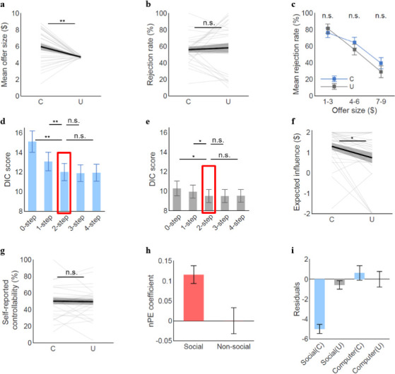
Figure 2—figure supplement 2. Rejection rates as a function of offer size.

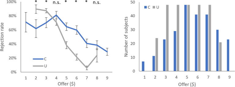
We reported and displayed the binned rejection rates mainly for two reasons: (1) It had a better matched subsample size for each bin and (2) the range of the offers were unmatched unintentionally for the fMRI sample ($1–9 for the Controllable condition; $2–8 for the Uncontrollable condition). (a) Rejection rates by each offer size show by and large consistent pattern with the binned results. (b) Participants distribution is depicted by each offer size. Note that a mixed-effect logistic regression, a statistically more stringent analysis, still shows consistent results with the binned results (Supplementary file 1). Error bars represent SEM; *p<0.05; C, controllable; fMRI, functional magnetic resonance imaging; n.s., not significant; U, Uncontrollable.

Figure 2—figure supplement 3. Response time.

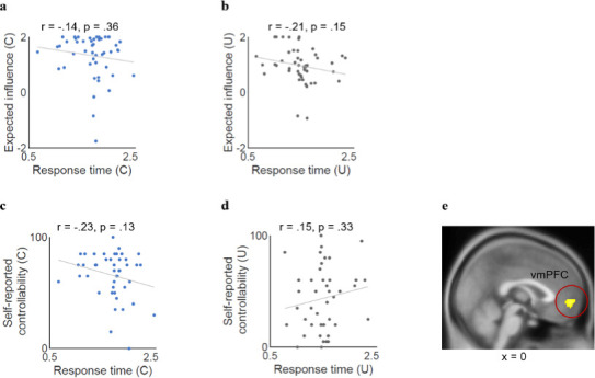
For neither condition, response times showed correlation (a, b) with expected influence, or (c, d) with self-reported controllability. Each dot represents a participant. (e) We also conducted fMRI analyses to include trial-by-trial RT as the first parametric regressor followed by our main parametric regressor (chosen values) in the original GLM. We did not find any significant neural activation in relation to the response time that survived the threshold of P_FDR<0.05. However, consistent with the result from the GLM without response times, the vmPFC chosen value signals were still significant at P_FDR<0.05 and k>50 after controlling for any potential RT effects (peak coordinate [0, 54, –2]). Error bars and shades represent EM. *p<0.05; **p<0.01; n.s. indicates not significant. For (a–d), each dot represents a participant. C, controllable; fMRI, functional magnetic resonance imaging; n.s., not significant; U, Uncontrollable; vmPFC, ventromedial prefrontal cortex.

Figure 2—figure supplement 4. Shift ratio.

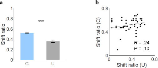
To examine whether participants behaved in a more habitual way in the Controllable condition, we analyzed the shift ratio of both conditions (i.e., the number of the trials where the choice was shifted from the previous trial divided by the total number of the trials). (a) We found that shift ratio was higher for the Controllable than the Uncontrollable condition (mean_C=52.5%, mean_U=36.2%, t(47)=6.62, p<0.001). (b) Shift ratio was not significantly correlated between the two conditions (r=0.24, p=0.10). Together with the RT analysis (Figure 2d), these results suggest that participants were less habitual and more deliberative in the Controllable condition.