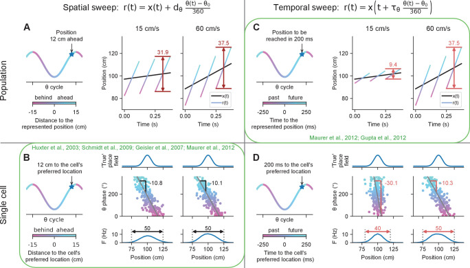
Figure 1. Simulated effect of running speed on population and single-cell properties in spatial sweep and temporal sweep models.

Certain findings in previous studies (green) paradoxically support the spatial sweep at the single-cell level, but the temporal sweep at the population level. (A) Left. At different phases of theta, the population represents positions shifted behind or ahead in space by fixed distances. Right. The black lines represents the rat’s actual location $x(t)$ as it runs through a linear track; the color-coded lines indicate theta trajectories represented by the place cell population $r(t)$. Since each theta trajectory starts and ends at fixed distances behind and ahead of the animal’s current location, the length of a theta trajectory increases slightly with running speed (37.5 vs. 31.9 cm) to account for the animal’s motion during the span of the theta cycle. (B) Left. At the single-cell level, the phases at which a cell spikes reflect the distances to the cell’s preferred location. Right. The cell’s preferred location is defined by its underlying 'true' place field (top). The cell fires proportionally to the activation of its true place field at $r(t)$, generating a phase precession cloud (middle) and corresponding measured place field (bottom). Phase precession slopes and place field sizes remain constant with running speed since, e.g., the cell always starts firing at 12 cm from the cell’s preferred location. (C) Left. At different phases of theta, the population represents the positions that were or will be reached at fixed time intervals into the past or future, respectively. Right. A higher running speed leads to a proportionally increased theta trajectory length since, e.g., the position that will be reached in 200 ms is further ahead in space at higher speeds. (D) Left. At the single-cell level, the phase of theta reflects the time to reach the cell’s preferred location. Right. At higher speed, the phase precession slope becomes shallower (−10.3 vs. −30.1 °/cm) and the size of the measured place field increases (50 vs. 40 cm) since, e.g., the cell will start signaling arrival at the cell’s preferred location in 200 ms from an earlier position in space.

Figure 1—figure supplement 1. Schematic illustration of the relationship between place fields, theta phase precession, and theta sequences.

Illustration of theta phase coding in spatial navigation. (A) A rat is running from left to right on a linear track. The firing rate of three place cells are indicated in different colors. (B) The idealized theta phase vs. position relationship for the spikes emitted by each of the cells shows a decrease in phase as the animal crosses the field (theta phase precession). (C) At the population level, phase precession manifests as spike sequences that represent, in a temporally compressed fashion, the sequence of place fields being traversed. The falling edge of the oscillation holds spikes from place cells with fields centered behind the current position of the rat, followed by spikes from cells with fields centered at the current position of the rat at the trough of the oscillation, and place cells with fields centered ahead in the rising edge.