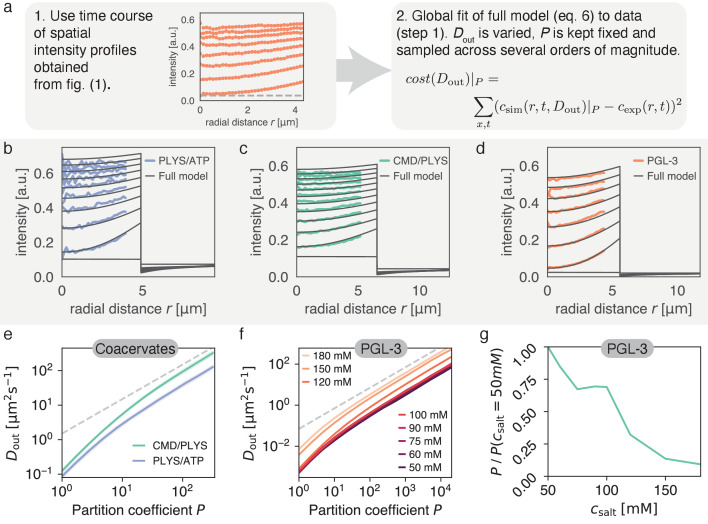
Figure 4. Varying partition coefficient $P$ and diffusivity outside $D_{\mathrm{out}}$ simultaneously can lead to similar recovery kinetics.

(a) Schematics of the fitting approach used to extract the relationship between $P$ and $D_{\text{out}}$. Although there is one specific pair ($P$, $D_{\text{out}}$) with the lowest cost (see Figure 5), there is a line in ($P$, $D_{\text{out}}$) space, which produces good fits for a range of values. (b) Spatial recovery of a single PLYS/ATP droplet (blue) with a fit to the full model (black). Note, data close to the droplet boundary cannot be fit, due to optical artefacts giving rise to an artificially broad interface (see Materials and methods and Figure 1a). (c) Same as (b) for a CMD/PLYS coacervate droplet. (d) Same as (b) for a PGL-3 droplet. (e) Given the partition coefficient $P$, $D_{\mathrm{out}}$ is found by fitting the coacervate data to the model. Note the convergence to a power law, $D_{\mathrm{out}}\propto P^n$ with $n=1$ for large partition coefficients (gray dashed line; for a discussion see Appendix 2). Shaded area around curves: standard deviation. Replicates: same as in Figure 1g. (f) Same as (e) but for PGL-3 with different salt concentrations. Note the order from top to bottom from highest to lowest salt concentration. (g) Based on (f), the change of partition coefficient $P(c_{\mathrm{salt}})$ can be estimated for a given $D_{\mathrm{out}}$. Confidence intervals not shown for clarity. Similar to panel e. Replicates: same as in Figure 1f.