Nonparametric estimation of distributions and diagnostic accuracy based on group-tested results with differential misclassification

Abstract

This article concerns the problem of estimating a continuous distribution in a diseased or nondiseased population when only group-based test results on the disease status are available. The problem is challenging in that individual disease statuses are not observed and testing results are often subject to misclassification, with further complication that the misclassification may be differential as the group size and the number of the diseased individuals in the group vary. We propose a method to construct nonparametric estimation of the distribution and obtain its asymptotic properties. The performance of the distribution estimator is evaluated under various design considerations concerning group sizes and classification errors. The method is exemplified with data from the National Health and Nutrition Examination Survey study to estimate the distribution and diagnostic accuracy of C-reactive protein in blood samples in predicting chlamydia incidence.

1 ∣. INTRODUCTION

A common objective in population health and health policy research is to estimate the prevalence, and identify potential predictors, of a disease, which is usually achieved by screening for the disease among a representative sample of the population. Because screening for the disease can be costly and time consuming, especially when the disease prevalence is low, group testing strategy has been advocated (Gastwirth and Hammick, 1989; Chen and Swallow, 1990; Tu et al., 1995; Hepworth, 1996; Hughes-Oliver and Rosenberger, 2000; McCann and Tebbs, 2007). Such a screening strategy was first introduced by Dorfman (1943) to test for syphilis antigen in the U.S. army recruit using pooled blood samples. With this strategy, blood samples from different subjects were pooled and tested. Subjects in a pool tested negative were declared free of infection, whereas retesting was subsequently performed on each subject in a pool that was tested positive. It is worth noting that while retesting is needed for screening for diseased subjects, it is not necessary for estimation of the disease prevalence.

Regression analysis has also received considerable attention to investigate the association of disease prevalence with interested covariates (Xie, 2001; Bilder and Tebbs, 2009; Delaigle and Meister, 2011; McMahan et al., 2013; Zhang et al., 2013; Wang et al., 2015). When disease occurrence is the result of an underlying time-to-event process, Petito and Jewell (2016) recently proposed a nonparametric maximum likelihood estimator of the time-dependent prevalence based on the group-tested data. In addition to saving cost and protecting confidentiality, group testing also has a somewhat counter-intuitive property. If classification error occurs in disease identification and the prevalence is low, then group testing may result in more precise estimator than individual testing for each subject; see Tu et al. (1995), Liu et al. (2012), Petito and Jewell (2016), Huang et al. (2017), among others.

The present paper concerns a different problem of estimating a continuous distribution in a diseased or nondiseased population when only group-based test results on the disease status are available. The context is that (a) only group-tested data of a disease are available; and (b) corresponding to each subject, concentration level of a continuous biomarker is observed. Our aim is to estimate the distribution of the biomarker given the disease status, and to make further inference such as constructing the receiver operating characteristic (ROC) curve to assess the diagnostic accuracy of the biomarker.

This research is partly motivated by mother-infant dyad studies to investigate whether a maternal biomarker can be used for diagnosis/classification of a disease for infants, for example, whether early pregnancy red cell folate levels indicates risk of having a child with neural tube defects (Milunsky et al., 1989). In such a study, the biomarker is measured on a continuous scale from individual mothers during their pregnancy. However, insufficient amount of blood from an infant may hinder individual testing for the disease. Instead, blood samples from a number of infants are pooled and screened for the disease. For this application, we are particularly interested in constructing the ROC curve of the maternal biomarker for diagnosis/classification of the disease for infants, which requires estimation of the distribution of the biomarker given disease status.

Similar data structure may be encountered even when both disease status and biomarker level are observed for each individual. For certain diseases such as sexually transmitted diseases (eg, chlamydia and HIV) and rare genetic mutations, it is imperative that patients’ confidentiality be protected. In this case, one appealing approach is to present disease statuses for groups, thus masking individual information on the disease (Gastwirth and Hammick, 1989). We will use the National Health and Nutrition Examination Survey study to demonstrate the problem and our methods. In the study, chlamydia infection was detected from urine sample and C-reactive protein (CRP) was measured from blood sample for each individual. Again, estimation of the distribution of CRP given infection status is of interest.

To the best of our knowledge, however, such a problem has not been addressed in the literature. The problem is challenging because individual disease statuses are not observed and group-tested results are often subject to misclassification. To further complicate the issue, misclassification rates may be differential, depending on the group size and the number of the diseased individuals in the group. We propose a method to construct nonparametric estimation of the distribution and obtain its asymptotic properties. We evaluate the performance of the distribution estimator under various design considerations concerning group sizes and classification errors. Along the way, we construct estimation of the ROC curves and the area under the curves.

The paper is organized as follows. Realizing that the nonparametric likelihood function is not identifiable with respect to the unknown prevalence and distributions, we present in Section 2 a shape-restricted two-step procedure to construct nonparametric estimators of the continuous distributions and derive their uniform consistencies and asymptotic distributions. Utilizing the estimated distributions, estimators for the ROC curve and its area are obtained, and their asymptotic distributions are established, in Section 3. Simulation studies are conducted in Section 4 to investigate the efficiency of the proposed method as compared to individual testing under various design considerations concerning group sizes and classification errors. In Section 5, we illustrate the methods with data on chlamydia and CRP from the National Health and Nutrition Examination Survey study. Some discussions are presented in Section 6. Proofs of the theorems are provided in the Web Appendix.

2 ∣. ESTIMATION METHODS

2.1 ∣. Notations and likelihood function

Consider a bivariate variable (X, D) where X is the concentration level of a continuous biomarker with distribution F and D indicates the true binary status of a disease (0 if disease-free and 1 if diseased) with prevalence p = Pr(D = 1). Let M be the observed diseased status from the assay, with specificity π₀ = Pr(M = 0∣D = 0) and sensitivity π₁ = Pr(M = 1∣D = 1), respectively. Our interest is in estimating the conditional distributions F₀(x) = Pr(X ≤ x ∣ D = 0) and F₁(x) = Pr(X ≤ x ∣ D = 1). (Note that F = (1 – p)F₀ + pF₁.)

Consider N subjects that are randomly divided into n groups of sizes K_i, i = 1,…, n, where K₁ + cdots + K_n = N. The continuous variable X is observed on each subject, yielding X_ik for the kth subject in the ith group, k = 1,…, K_i, i = 1,…, n. Denote ${\mathcal{X}}_i=(X_{i1},\dots ,X_{i{K}_i}{)}^T$ for i = 1,…, n, where the symbol “T” represents the transpose of a vector or matrix. Instead of individual-tested results, group-tested results, represented by {${\tilde{M}}_i$, i = 1,…, n}, are available. Let D_ij be the true disease status of the jth subject in the ith group and define ${\tilde{D}}_i=\max \{D_{i1},\dots ,D_{i{K}_i}\}$. For each group i, we assume that the specificity of the test remains unchanged, that is, $\text{Pr}({\tilde{M}}_i=0\mid {\tilde{D}}_i=0)={\pi }_0$, while the sensitivity is differential, depending on the group size K_i and the number d_i of diseased subjects in the group, that is, $\text{Pr}({\tilde{M}}_i=1\mid {\tilde{D}}_i=1)={\pi }_1^{\ast }(K_i,d_i)$. Throughout we assume that the specificity π₀ and sensitivity π₁ are known, and the sensitivity ${\pi }_1^{\ast }$ is a given function of d and K, where d is the number of diseased subjects in a group and K is the group size. In general, ${\pi }_1^{\ast }$ increases in d for given K, whereas decreases in K for given d. When K =1, ${\pi }_1^{\ast }$ becomes π₁. Moreover, when a group consists of entirely diseased subjects, that is, d = K, the sensitivity is not influenced by dilution, hence ${\pi }_1^{\ast }={\pi }_1$.

Let f₁(x) and f₀(x) be the density function corresponding to F₁(x) and F₀(x), respectively. Throughout, we assume that given the true disease status ${\tilde{D}}_i$, the biomarker levels ${\mathcal{X}}_i$ of the subjects in the group and the group-tested result ${\tilde{M}}_i$ are independent. Thus, $f(\mathcal{X}\mid \tilde{M}=m,\tilde{D}=d)=f(\mathcal{X}\mid \tilde{D}=d)$, where m = 0, 1 and d = 0, 1. Denote by $f({\mathcal{X}}_i,{\tilde{M}}_i)$ the joint density of ${\mathcal{X}}_i$ and ${\tilde{M}}_i$. Then it follows that the likelihood function for the observations $\{({\mathcal{X}}_i^T,{\tilde{M}}_i{)}^T:i=1,\dots ,n\}$ is given by

$$L=\prod _{i=1}^{n}f({\mathcal{X}}_i,{\tilde{M}}_i=0{)}^{I({\tilde{M}}_i=0)}\prod _{i=1}^{n}f({\mathcal{X}}_i,{\tilde{M}}_i=1{)}^{I({\tilde{M}}_i=1)},$$ (1)

where I(·) is an indicator function, $f({\mathcal{X}}_i,{\tilde{M}}_i=1)={\prod }_{k=1}^{K_i}\{p{f}_1(X_{ik})+(1-p)f_0(X_{ik})\}-f({\mathcal{X}}_i,{\tilde{M}}_i=0)$, and

$$\begin{gathered} f({\mathcal{X}}_i,{\tilde{M}}_i=0) \\ ={\pi }_0(1-p{)}^{K_i}\prod _{k=1}^{K_i}{f}_0(X_{ik})+\sum _{\begin{array}{c}\hfill l_1,\dots ,l_{K_i}=0\hfill \\ \hfill l_1+\cdots +l_{K_i}=d_i>0\hfill \end{array}}^1 \\ \times \left\{\prod _{k=1}^{K_i}{f}_0(X_{ik}{)}^{1-l_k}{f}_1(X_{ik}{)}^{l_k}\right\} \\ \times \{1-{\pi }_1^{\ast }(K_i,d_i)\}{p}^{d_i}(1-p{)}^{K_i-d_i} \end{gathered}$$

whose derivation is given in Web Appendix A.

2.2 ∣. A nonparametric estimation method

In what follows, we propose a nonparametric approach to estimating F₀ and F₁ based on the available data. For simplicity, we consider equal group sizes, that is, K₁ = ⋯ = K_n = N/n ≜ K; the results to be derived below can be straightforwardly extended to the situation where group sizes vary.

We first note that, if the forms of the two density functions are totally unspecified, then there exist distinct estimators of f₀ and f₁, as well as the prevalence p that yield the same likelihood, due to the mixture of f₀ and f₁ with an unknown proportion in each group; see proof in Web Appendix B. It is therefore infeasible to estimate F₀ and F₁ by directly maximizing the nonparametric likelihood function. We instead develop a two-step procedure that first estimates the distribution functions F(x) = Pr(X ≤ x), $F(x,\tilde{M}=0)=\text{Pr}(X\le x,\tilde{M}=0)$ and the prevalence p and then deduces the non-parametric estimators of F₁ and F₀ from the resulting estimators. Subsequently, a shape-restricted procedure is employed to improve the initial empirical estimators.

The number of groups that are tested positive, $n_1={\sum }_{i=1}^n{\tilde{M}}_i$, follows a binomial distribution with size n and probability

$$p_1=(1-{\pi }_0)(1-p{)}^K+\sum _{d=1}^K{\pi }_1^{\ast }(K,d)C_K^d{p}^d(1-p{)}^{K-d},$$

where $C_K^d$ represents the binomial coefficient “K choose d.” Let p₀ = 1 – p₁ and n₀ = n – n₁. It follows that the loglikelihood function based on the group testing results is l_G = n₀ log(p₀) + n₁ log(p₁). Then the maximum likelihood estimate $\widehat{p}$ of p is obtained by maximizing l_G. By the asymptotic normality of maximum likelihood estimator (van der Vaart, 1998), the estimator $\widehat{p}$ is asymptotically normal with mean p and variance

$$\begin{gathered} \text{var}(\widehat{p})=\frac{p_1(1-p_1)}{n}\{K(1-{\pi }_0)(1-p{)}^{K-1}\phantom{\}} \\ -{\phantom{\{}\sum _{d=1}^K{\pi }_1^{\ast }(K,d)C_K^d{p}^{d-1}(1-p{)}^{K-1-d}(d-Kp)\}}^{-2}. \end{gathered}$$

Empirical estimators of F(x) and $F(x,\tilde{M}=0)$ can be constructed, respectively, using all X-observations and the X-observations on the subjects in the groups that are tested negative. This yields

$$\begin{gathered} \tilde{F}(x)=\frac{1}{nK}\sum _{i=1}^n\sum _{k=1}^{K}I(X_{ik}\le x), \\ \tilde{F}(x,\tilde{M}=0)=\frac{1}{nK}\sum _{i=1}^{n}I({\tilde{M}}_i=0)\left\{\sum _{k=1}^{K}I(X_{ik}\le x)\right\}, \end{gathered}$$

respectively. Let $\mathcal{X}=(X_1,\dots ,X_K{)}^T$ be the concentration levels of the K subjects in a group, with true disease status (D₁,…, D_K)^T. Then due to the independence between $\mathcal{X}$ and $\tilde{M}$ conditional on (D₁,…, D_K), it follows that

$$\begin{gathered} F(x,\tilde{M}=0)=\text{Pr}(X_1\le x,D_1=0,\tilde{M}=0) \\ +\text{Pr}(X_1\le x,D_1=1,\tilde{M}=0) \\ =\text{Pr}(D_1=0,\tilde{M}=0)F_0(x) \\ +\text{Pr}(D_1=1,\tilde{M}=0)F_1(x), \end{gathered}$$

where

$$\begin{gathered} \text{Pr}(D_1=0,\tilde{M}=0) \\ =\text{Pr}(D_1=0,\max \{D_2,\dots ,D_K\}=0,\tilde{M}=0) \\ +\text{Pr}(D_1=0,\max \{D_2,\dots ,D_K\}=1,\tilde{M}=0) \\ ={\pi }_0(1-p{)}^K+\sum _{d=1}^{K-1}\{1-{\pi }_1^{\ast }(K,d)\}{C}_{K-1}^d{p}^d(1-p{)}^{K-d} \end{gathered}$$

and similarly $\text{Pr}(D_1=1,\tilde{M}=0)=\sum _{d=0}^{K-1}\{1-{\pi }_1^{\ast }(K,d+1)\}{C}_{K-1}^d{p}^{d+1}(1-p{)}^{K-1-d}$.

With the estimators $\widehat{p}$, $\tilde{F}(x)$, and $\tilde{F}(x,\tilde{M}=0)$, we obtain the nonparametric estimators of F₁(x) and F₀(x) as

$$\begin{gathered} {\tilde{F}}_0(x)=\frac{\widehat{p}\tilde{F}(x,\tilde{M}=0)-{\widehat{\gamma }}_1\tilde{F}(x)}{{\widehat{\gamma }}_2\widehat{p}-{\widehat{\gamma }}_1(1-\widehat{p})}, \\ {\tilde{F}}_1(x)=\frac{{\gamma }_2\tilde{F}(x)-(1-\widehat{p})\tilde{F}(x,\tilde{M}=0)}{{\widehat{\gamma }}_2\widehat{p}-{\widehat{\gamma }}_1(1-\widehat{p})}, \end{gathered}$$

where

$$\begin{gathered} {\widehat{\gamma }}_1=\sum _{d=0}^{K-1}\left\{1-{\pi }_1^{\ast }(K,d+1)\right\}{C}_{K-1}^d{\widehat{p}}^{d+1}(1-\widehat{p}{)}^{K-1-d}, \\ {\widehat{\gamma }}_2={\pi }_0(1-\widehat{p}{)}^K+\sum _{d=1}^{K-1}\left\{1-{\pi }_1^{\ast }(K,d)\right\}{C}_{K-1}^d{\widehat{p}}^d(1-\widehat{p}{)}^{K-d}. \end{gathered}$$

Similar to the conventional empirical distribution functions, ${\tilde{F}}_0$ and ${\tilde{F}}_1$ are step functions but not always with positive jumps at the data points. Although the empirical estimators ${\tilde{F}}_0$ and ${\tilde{F}}_1$ are consistent, they may not satisfy the requirements of a cumulative distribution function: being nondecreasing and between 0 and 1. To overcome this issue, we propose restricted estimators for F₀ and F₁ by imposing monotonicity on the empirical estimators. The new estimators of F₀ and F₁ are obtained by minimizing

$$\begin{gathered} \int {\left\{U(x)-{\tilde{F}}_0(x)\right\}}^{2}d{\tilde{F}}_0(x) \\ =\frac{1}{nK}\sum _{i=1}^n\sum _{k=1}^K{\left\{U(X_{ik})-{\tilde{F}}_0(X_{ik})\right\}}^2 \end{gathered}$$ (2)

and

$$\begin{gathered} \int {\left\{U(x)-{\tilde{F}}_1(x)\right\}}^{2}d{\tilde{F}}_1(x) \\ =\frac{1}{nK}\sum _{i=1}^n\sum _{k=1}^K{\left\{U(X_{ik})-{\tilde{F}}_1(X_{ik})\right\}}^2 \end{gathered}$$ (3)

over all cumulative distribution functions {U(x)}, respectively. Denote the minimizers of (2) and (3) by ${\tilde{F}}_0^{\ast }(x)$ and ${\tilde{F}}_1^{\ast }(x)$, which are referred to as the constrained empirical estimators of F₀(x) and F₁(x), respectively. By the projection theorem (see Proposition 2.2.1 of Bertsekas, 2003), the proposed estimators ${\tilde{F}}_0^{\ast }(x)$ and ${\tilde{F}}_1^{\ast }(x)$ are uniquely defined.

Moreover, ${\tilde{F}}_0^{\ast }$ and ${\tilde{F}}_1^{\ast }$ can be regarded as the isotonic regression or projection of the sets of points $\{{\tilde{F}}_0(X_{ik}):i=1,\dots ,n,k=1,\dots ,K\}$ and $\{{\tilde{F}}_1(X_{ik}):i=1,\dots ,n,k=1,\dots ,K\}$ with equal weight, respectively (Barlow et al., 1972; Robertson et al., 1988). To ensure the distribution function estimators lie between 0 and 1, ${\widehat{F}}_0(x)=\text{min}\{\max \{{\tilde{F}}_0^{\ast }(x),0\},1\}$ and ${\widehat{F}}_1(x)=\text{min}\{\max \{{\tilde{F}}_1^{\ast }(x),0\},1\}$ are used as the final estimators for F₀(x) and F₁(x), respectively.

Next, we establish the asymptotic properties of the proposed nonparametric distribution function estimators. By the aid of the isotonic regression properties, we first derive uniform consistency of ${\widehat{F}}_0$ and ${\widehat{F}}_1$. In what follows, the symbol $‘‘\stackrel{d}{\to }’’$ represents “converges weakly to” for a random process or “converges in distribution to” for a random variable, and $‘‘\stackrel{a.s.}{\to }’’$ means “converges almost surely” for a random variable. Then we define β₀(F) = sup{x : F(x) = 0} and β₁(F) = inf{x : F(x) = 1}. Assume that F₀ and F₁ have the same support, denoted by ${\mathcal{R}}_F=[{\beta }_0(F),{\beta }_1(F)]$.

Theorem 1 (Uniform consistency). Assume that 0 < p < 1, the group size K is fixed, and the specificity π₀, sensitivity π₁, and sensitivity function ${\pi }_1^{\ast }$ are known. Then as n → ∞,

$$\underset{x\in {\mathcal{R}}_F}{\text{sup}}\mid {\widehat{F}}_0(x)-F_0(x)\mid \stackrel{a.s.}{\to }0and\underset{x\in {\mathcal{R}}_F}{\text{sup}}\mid {\widehat{F}}_1(x)-F_1(x)\mid \stackrel{a.s.}{\to }0.$$

This theorem is a direct consequence of the properties of isotonic regression and the uniform laws of large numbers. If β₀(F) and β₁(F) are both finite, that is, −∞ < β₀(F) < β₁(F) < ∞, then the asymptotic normality of ${\widehat{F}}_0(x)$ and ${\widehat{F}}_1(x)$ can be established.

Theorem 2 (Asymptotic normality). Assume that F₀(x) and F₁(x) are both twice continuously differentiable. Denote the second derivative of F_υ(x) by $f_v^{\prime }(x)$ for υ = 0, 1. Let 0 < p < 1 and the group size K be fixed. Further assume that the specificity π₀, sensitivity π₁, and sensitivity function ${\pi }_1^{\ast }$ are known, and

$${\lambda }_0(F_0)=\frac{\underset{x\in {\mathcal{R}}_F}{\text{sup}}\mid f_0^{\prime }(x)\mid }{\underset{x\in {\mathcal{R}}_F}{\text{inf}}{f}_0^2(x)}<\infty and{\lambda }_1(F_1)=\frac{\underset{x\in {\mathcal{R}}_F}{\text{sup}}\mid f_1^{\prime }(x)\mid }{\underset{x\in {\mathcal{R}}_F}{\text{inf}}{f}_1^2(x)}<\infty .$$

Then as n → ∞,

$$\sqrt{n}\left(\begin{array}{c}\hfill {\widehat{F}}_0(x)-F_0(x)\hfill \\ \hfill {\widehat{F}}_1(x)-F_1(x)\hfill \end{array}\right)\stackrel{d}{\to }\left(\begin{array}{c}\hfill K_{F_0}(x)\hfill \\ \hfill K_{F_1}(x)\hfill \end{array}\right),$$

in $D({\mathcal{R}}_F{)}^2=D({\mathcal{R}}_F)\times D({\mathcal{R}}_F)$, where $D({\mathcal{R}}_F)$ are functions on ${\mathcal{R}}_F$ that are right continuous with left-side limits, (K_F0(x), K_F1(x))^T is a vector of mean zero Gaussian process with continuous paths and the covariance function given in the Web Appendix.

3 ∣. ROC CURVES ANALYSIS AND DIAGNOSTIC ACCURACY

With the distribution function estimators ${\widehat{F}}_0$ and ${\widehat{F}}_1$, various statistical inferences can be made. Here we utilize the distribution estimators for ROC curves analysis. The ROC curve is a fundamental tool in the assessment of biomarkers in diagnostic medicine and many other areas; see Zhou et al. (2011). The ROC curve of X with respect to D is given by $\text{ROC}(u)=1-F_1(F_0^{-1}(1-u))$ for u ∈ [0, 1] and the area under the ROC curve is $\text{AUC}={\int }_0^1\text{ROC}(u)du$. With ${\widehat{F}}_0$ and ${\widehat{F}}_1$ obtained in Section 2.2, the estimators of ROC(u) and AUC can be naturally obtained as

$$\begin{gathered} \widehat{\text{ROC}}(u)=1-{\widehat{F}}_1\left({\widehat{F}}_0^{-1}(1-u)\right), \\ u\in [0,1]\text{and}\widehat{\text{AUC}}={\int }_0^1\widehat{\text{ROC}}(u)du. \end{gathered}$$

The asymptotic distributions of $\widehat{\text{ROC}}(u)$ and $\widehat{\text{AUC}}$ are given in the following theorem.

Theorem 3. Assume the conditions in Theorem 2 hold and for υ = 0, 1, f_υ(x) is positive on [$F_v^{-1}(a)-ϵ$, $F_v^{-1}(b)+ϵ$] for some 0 < a < b < 1 and ϵ > 0. Then, as n → ∞,

$$\begin{gathered} \sqrt{n}\left\{\widehat{ROC}(u)-ROC(u)\right\} \\ \stackrel{d}{\to }{K}_{F_0}(F_0^{-1}(1-u))\frac{f_1(F_0^{-1}(1-u))}{f_0(F_0^{-1}(1-u))}-K_{F_1}(F_0^{-1}(1-u)) \end{gathered}$$

for u ∈ [1 – b, 1 – a] and

$$\sqrt{n}(\widehat{AUC}-AUC)\stackrel{d}{\to }{\int }_{-\infty }^{\infty }\left\{K_{F_0}(x)\frac{f_1(x)}{f_0(x)}-K_{F_1}(x)\right\}d{F}_0(x),$$

where (K_F0(x), K_F1(x))^T is a vector of mean zero Gaussian process with continuous paths defined in Theorem 2.

4 ∣. SIMULATIONS

We conducted extensive simulation studies to investigate the performance of our proposed nonparametric estimators of continuous distribution functions based on group-tested results, as compared to estimators with individual-tested results of all nK subjects and a random sample of size n from the nK subjects, termed herein as full individual testing and random individual testing, respectively. We present the results for the former here; the results for the latter are presented in Web Appendix D.

The common group size K was chosen from {1, 2, 5, 10}. The values of specificity π₀ and sensitivity π₁ were chosen from {0.80, 0.90, 0.95, 1.00}. We use the model considered by Hung and Swallow (1999) to specify ${\pi }_1^{\ast }={\pi }_{1}d∕\{d+\lambda (K-d)\}$, where λ is a constant set to be 0.02. The prevalence p was selected from {0.02, 0.05}, reflecting the incidence of a rare disease. For a given (total) sample size N = nK, a random sample of $({\mathcal{X}}^T,\tilde{M}{)}^T$ was produced as follows, where, as previously defined, $\tilde{M}$ is the test result on the group, and $\mathcal{X}$ is the vector of individual X-values. First, we generated the true disease status {D_ik : 1 ≤ i ≤ n; 1 ≤ k ≤ K} from a Bernoulli distribution with probability p. The corresponding X-values were generated from LN (1, 1.44) for subjects with D = 1, and LN(0,1) for other subjects, where LN(μ, σ²) stands for the distribution function of a random variable whose logarithm follows a normal distribution with mean μ and variance σ². Second, the N subjects were randomly divided into n groups each with size K. For a group with all D = 0, its corresponding group-tested result ($\tilde{M}$) was generated from a Bernoulli distribution with probability 1 – π₀; otherwise, the test result was generated from a Bernoulli distribution with probability ${\pi }_1^{\ast }$.

In what follows, we assess the finite-sample performance of the proposed estimation approach for various group sizes and numbers of groups. The evaluations are carried out based on three commonly used criteria including the integrated absolute bias, root integrated mean squared error, and the average pointwise 95% coverage probability. For an estimator $\widehat{F}(x)$ of a function F(x), its integrated absolute bias is defined as $\int \mid E\{\widehat{F}(x)-F(x)\}\mid dx$, and its root integrated mean squared error is defined as $[\int E\{\widehat{F}(x)-F(x){\}}^{2}dx{]}^{1∕2}$. The integrals for the two indexes are computed using a Riemann sum over selected quantiles of F determined by 50 equally spaced points in {1/50,…, 1}. The expectations in the integrals were approximated using Monto Carlo simulation. The average pointwise coverage probability is computed as the average of the coverage probabilities of the 50 confidence intervals with 95% nominal level over the same grids. We used the bootstrap procedure that resamples the group-level observations $\{({\mathcal{X}}_i^T,{\tilde{M}}_i{)}^T:i=1,\dots ,n\}$ with replacement to estimate the coverage probability. Throughout, 1000 Monto Carlo simulations are conducted. For each simulation, 1000 bootstrap replicates are generated to estimate the coverage probability of a confidence interval. For a rare disease, the number of disease-free subjects in groups tested negative tends to be large. This ensures relatively accurate estimate of F₀ for low to moderate misclassification rates. For this reason, we report only simulation findings on F₁; results on F₀ are presented in Web Appendix D.

For the comparison between group testing and full individual testing, we set the total number of subjects to be N = 10 000. Table 1 presents the finite sample performance of ${\widehat{F}}_1$ as compared to that of estimators with individual-tested results on nK subjects, in terms of the aforementioned three measures. As anticipated, the estimator tends to underperform when the prevalence is low and misclassification exists. This is mainly because the number of groups tested positive can be quite small when the prevalence is very low. For example, when p = 0.02, the expected number of subjects with disease is 100 and the expected number of groups of size 10 tested positive reduces to 91. As the prevalence increases or the misclassification rate decreases, the performance of ${\widehat{F}}_1$ improves with smaller integrated absolute bias and root integrated mean squared error, and larger coverage probability; with P = 0.05, the average coverage probabilities get much closer to the 95% nominal level.

TABLE 1.

Finite sample performance of ${\widehat{F}}_1$ in terms of integrated absolute bias (IAB), root integrated mean squared error (RIMSE), and 95% coverage probability (CP) for fixed sample size N = 10 000 (K is the group size)

		p = 0.02			p = 0.05
(π0, π1)	K	IAB	RIMSE	CP	IAB	RIMSE	CP
(0.90, 0.90)	1	0.0033	0.2829	87.4%	0.0032	0.1212	92.1%
	2	0.0028	0.2609	90.7%	0.0033	0.1286	92.6%
	5	0.0034	0.2819	91.4%	0.0029	0.1577	93.1%
	10	0.0045	0.3378	91.6%	0.0028	0.2177	92.7%
(1.00, 1.00)	1	0.0013	0.1187	94.8%	0.0013	0.0758	95.3%
	2	0.0018	0.1386	94.5%	0.0033	0.0862	94.9%
	5	0.0034	0.1850	92.8%	0.0022	0.1217	94.2%
	10	0.0015	0.2509	92.0%	0.0014	0.1700	93.8%

The pointwise efficiency of group testing relative to individual testing is displayed in Figure 1 for selected values of prevalence and diagnostic error. The vertical axis in the figure is the log2-ratio of the variance of ${\widehat{F}}_1(x)$ from group testing relative to that from individual testing; a negative log2-ratio value at some x indicates better performance of group testing than individual testing at x. For p = 0.02 and the specificity and sensitivity less than 1, we observe that the variances of ${\widehat{F}}_1$ from group testing are generally smaller than those from individual testing, especially for large x-values. However, such superiority disappears if there is no diagnostic error. For P = 0.05, the trend is similar but with larger log2-ratios of variance than for P = 0.02.

FIGURE 1.

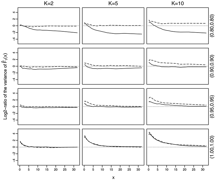
Pointwise relative efficiency of ${\widehat{F}}_1(x)$ based on group-tested results to individual-tested results. The solid lines are for P = 0.02 and the dashed lines are for P = 0.05

The overall relative efficiency, defined here as the log2-ratio of the integrated mean squared error of ${\widehat{F}}_1$ using group-tested results as compared with using individual-tested results, are displayed in Figure 2 for p ∈ [0, 0.3]. The figure shows that the log2-ratio of variances is increasing with prevalence, starting with being negative and then becoming positive. This implies that the distribution function estimator based on group-tested results is more efficient than that based on individual-tested results when the prevalence is below a certain threshold, and less efficient otherwise. The threshold appears to vary as group size changes; in our case, the threshold is found to be 0.05, 0.03, and 0.02 for K = 2, 5, and 10, respectively.

FIGURE 2.

Overall relative efficiency of ${\widehat{F}}_1$ based on group-tested results to individual-tested results with π₀ = π₁ = 0.90

5 ∣. APPLICATIONS

We exemplify our proposed estimation method with data from the National Health and Nutrition Examination Survey study (NHANES; https://www.cdc.gov/nchs/nhanes/index.htm), a very large population-based study designed to assess the health and nutritional status of adults and children in the United States.

In the NHANES study, tests for genital chlamydia infections are performed on urine samples from the study participants by the DNA strand displacement amplification method, which is a mainstay assay technique. The strand displacement amplification has been estimated to have a specificity of π₀ = 0.99 and a sensitivity of π₁ = 0.90 (Haugland et al., 2010). The publicly released chlamydia data include assay results of eligible participants aged 18-39. Chlamydia, as one of the most common sexually transmitted disease, is caused by chlamydia trachomatis, an intracellular bacteria that can stimulate the change of the levels of inflammatory markers, such as erythrocyte sedimentation rate and CRP (Łój et al., 2016; Park et al., 2017). Here for illustration, we consider using CRP ranging from 0.01 to 2.34 as the biomarker for chlamydia; thus M is the indicator of presence of chlamydia in the urine specimen and X is the CRP in the blood specimen of a participant.

We focus on the chlamydia and CRP data between 1999 and 2010 that were collected from six consecutive and independent surveys (NHANES 1999-2000, 2001-2002, 2003-2004, 2005-2006, 2007-2008, and 2009-2010). Due to public health interest of certain population subgroups (eg, Hispanic and Asian), the NHANES sampled larger numbers of these subgroups. To eliminate the effects of oversampling and complex survey design, we resampled with replacement the data from each two-year survey dataset, with probability proportional to the sampling weights; the sample size was set to be the same as that of the original dataset. Then we combined the resulted samples to form a large sample. After removing the subjects with missing values of chlamydia or CRP, N = 12 330 independent observations of (X, M)^T are included in the final analysis dataset, out of which 218 subjects were tested positive for chlamydia. Note that although the NHANES did not employ group testing for detecting chlamydia, it suffices to exemplify our methods by constructing group-based data. As chlamydia and CRP are assayed using different specimens, it allows us to create group-tested results for the presence of chlamydia independently by treating the testing results available in the current dataset as the subjects’ true disease statuses and then randomly assigning the urine specimens into groups of sizes K, while maintaining the individual observations of CRP. The true disease status of a group was positive if at least one subject had a positive result. With these data, group-tested results are then obtained for the presence of chlamydia by using 1 – π₀ and ${\pi }_1^{\ast }(K,d)$ as the corresponding Bernoulli success probabilities. The rationale behind this is that investigators may only be willing to provide group-tested results in order to protect subjects’ confidentiality.

Our goal is to estimate the distribution function of CRP in the noninfected and infected population, and investigate the diagnostic ability of CRP as a biomarker for chlamydia by constructing the ROC curve. For comparative purpose, we also calculate the estimators based on the individual-tested data where the disease status of study participants are fully observed. Likewise, we assume that ${\pi }_1^{\ast }(K,d)={\pi }_{1}d∕\{d+\lambda (K-d)\}$ with λ = 0.02 for illustration. Figure 3A displays four estimates of the distribution function F₁ of CRP in the population aged 18-39 with infection of chlamydia for group size of 1, 2, 5, and 10. From this figure, it can be seen that the estimates based on group-tested data with K = 2 and K = 5 are similar to that from the individual-tested data, except when the value of F₁(x) is large. Due to the large sample size and low prevalence, the estimates of F₀ for all considered group sizes are almost the same and we therefore omit the displays here.

FIGURE 3.

A Estimates of distribution function of CRP in the population aged 18-39 with chlamydia; B estimates of ROC curve of CRP as a biomaker for chlamydia based on the population aged 18-39. The specificity and sensitivity are π₀ = 0.99 and π₁ = 0.90

With the distribution estimators, we estimate the ROC curves of CRP based on both group-tested data and individual-tested data, and present the curves in Figure 3B. Likewise, the ROC curves for K = 1, K = 2, and K = 5 are quite similar and differ from the others. To compare the efficiency of the estimates, we computed 95% confidence bands of the ROC curve estimates based on 1000 bootstrap replicates; the results are presented in Web Appendix E. Overall, the variance of ROC curve estimates for K = 2 is the smallest among the four estimates. It indicates that the estimate based on group-tested data with K = 2 yields similar estimate to that from the individual-tested data. Such a finding is further strengthened by the area under the estimated ROC curves, which are 0.575, 0.547, 0.556, and 0.634 with standard errors of 0.037, 0.029, 0.054, and 0.071, respectively, for K = 1, 2, 5, and 10.

6 ∣. DISCUSSION

In this work, we considered the problem of estimating the distribution of a continuous biomarker when only group-based test results on the disease status are available. Due to nonidentifiability of the nonparametric MLEs, we proposed a two-step procedure to construct nonparametric estimation of the continuous distribution given the disease status and established consistency and asymptotic normality. By imposing certain constraints, such as parametric/semiparametric models, on the distributions, the issue of nonidentifiability can be avoided and the maximum likelihood estimation can be implemented; see, among others, recent work of Li et al. (2017). Further research is needed along these lines for group-tested data.

ROC curves were also constructed to assess the diagnostic accuracy of the biomarker for the disease. Simulation studies demonstrated that group-tested results can yield more efficient distribution estimation than individual-tested results when the disease has a low prevalence and its detection is associated with misclassification. Similar conclusions were reached concerning comparison of group-tested results with individual-tested results by Tu et al. (1995) and Liu et al. (2012) for estimation of the disease prevalence and by Petito and Jewell (2016) for estimation of the time-dependent prevalence.

An alternative method for estimating the distribution functions from group testing data is to use the Bayes’s formula. To be specific, one can first estimate Pr(D = 1 ∣ X = x), p, and f(x) separately, and then obtain the estimators for the disease-specific density functions Pr(X = x ∣ D = 1) and Pr(X = x ∣ D = 0) through the Bayes’s formula, where f(x) is the density function of X. The distribution function estimators can then be derived by integrating the normalization of the resulted density estimators. The density function f(x) can be estimated by its empirical density function, and the prevalence p can be estimated using the method in Tu et al. (1995) and Liu et al. (2012). For the conditional probability Pr(D = 1∣X = x), most existing methods were developed based on parametric models, where the shape of the regression curve is assumed to be known. Delaigle and Meister (2011) proposed a nonparametric estimator based on a kernel method. But their estimator requires selecting a tuning parameter (bandwidth), which is usually not easy to determine in practice. Moreover, their method was designed for assays without classification errors, although an extension to the case where the observations are subject to misclassification is briefly discussed in their paper. Further research is needed along this line.

In constructing the estimators and establishing their asymptotic properties, we assume that the sensitivity and specificity of the assay used to detect the disease are known and differential. Although in many applications these assumptions are reasonable, in many others they may be violated (Hwang, 1976; McMahan et al., 2013). For the applications where the specificity and sensitivity are unknown, one can use a validation sample to estimate the classification errors of the imperfect assay, when a gold standard (a perfect assay/test) is available. For example, the Western blot test, which is more accurate and more expensive than the ELISA, is usually regarded as a gold standard for HIV testing (Johnson and Gastwirth, 2000). The estimated sensitivity and specificity from the validation study are assumed a priori, and subsequently the estimates of the disease prevalence and biomarker distributions can be derived using the proposed methods.

Although the present paper focuses on a single biomarker, it is foreseeable that multiple biomarkers may be measured, either cross-sectionally or longitudinally. A problem of particular interest is to combine these biomarkers to improve the diagnostic accuracy of the disease by achieving higher ROC curves or larger area under the ROC curves (Su and Liu, 1993; Liu et al., 2005). It appears challenging to address such a problem, even when considering only linear combinations of the biomarkers.

Multiplex assays, which test for multiple diseases simultaneously, have been increasingly used in real applications to reduce the cost and time; for example, the Procleix Ultrio Assay has been used for simultaneously testing for HIV, hepatitis B, and hepatitis C. Some work has been done on investigating the use of group testing with multiplex assays (Tebbs et al., 2013; Hou et al., 2017; Bilder et al., 2019), focusing on case identification. It is of interest to consider the problem of estimating the distribution function of a continuous biomarker when the disease status is determined using the tools of group testing and multiplex assays.

It is common to include potential confounding factors in real applications, especially observational studies. We suggest the following strategy to incorporate covariate adjustment by extending the proposed method to obtain covariate-adjusted estimates. For a covariate Z at z, one can first derive a nonparametric estimator ${\widehat{F}}_i(x,z)$ of the joint disease-specific distribution function, F_i(x, z), i = 0, 1, of the biomarker and the covariate. This can be done by extending the proposed method in the present article for a univariate distribution to multivariate distribution, but more tedious technical derivations and extensive numerical computations are expected. Subsequently, for each disease status i = 0, 1, a nonparametric estimator ${\widehat{F}}_i(x\mid Z=z)$ of the conditional distribution function F_i(x ∣ Z = z) of the biomarker given the covariate can be constructed. These estimates of conditional distributions can then be used to obtain estimates of the (covariate-adjusted) ROC curve and its area. Further research is needed to investigate the performance of this (or perhaps other) strategies.

REFERENCES

- Barlow RE, Bartholomew DW, Bremner JM and Brunk HD (1972) Statistical Inference under Restrictions: The Theory and Application of Isotonic Regression. New York, NY: Wiley. [Google Scholar]
- Bertsekas DP (2003) Convex Analysis and Optimization. Belmont, MA: Athena Scientific. [Google Scholar]
- Bilder CR and Tebbs JM (2009) Bias, efficiency, and agreement for group-testing regression models. Journal of Statistical Computation and Simulation, 79, 67–80. [DOI] [PMC free article] [PubMed] [Google Scholar]
- Bilder CR, Tebbs JM and McMahan CS (2019) Informative group testing for multiplex assays. Biometrics, 75, 278–288. [DOI] [PMC free article] [PubMed] [Google Scholar]
- Chen CL and Swallow WH (1990) Using group testing to estimate a proportion, and to test the binomial model. Biometrics, 46, 1035–1046. [PubMed] [Google Scholar]
- Delaigle A and Meister A (2011) Nonparametric regression analysis for group testing data. Journal of the American Statistical Association, 106, 640–650. [DOI] [PMC free article] [PubMed] [Google Scholar]
- Dorfman R (1943) The detection of defective members of large populations. Annals of Mathematical Statistics, 14, 436–440. [Google Scholar]
- Gastwirth JL and Hammick PA (1989) Estimation of prevalence of a rare disease, preserving anonymity of subjects by group testing: application to estimating the prevalence of aids antibodies in blood donors. Journal of Statistical Planning and Inference, 22, 15–27. [Google Scholar]
- Haugland S, Thune T, Fosse B, Wentzel-Larsen T, Hjelmevoll SO and Myrmel H (2010) Comparing urine samples and cervical swabs for chlamydia testing in a female population by means of strand displacement assay (SDA). BMC Womens Health, 10. 10.1186/1472-6874-10-9 [DOI] [PMC free article] [PubMed] [Google Scholar]
- Hepworth G (1996) Exact confidence intervals for proportions estimated by group testing. Biometrics, 52, 1134–1146. [Google Scholar]
- Hou P, Tebbs JM, Bilder CR and McMahan CS (2017) Hierarchical group testing for multiple infections. Biometrics, 73, 656–665. [DOI] [PMC free article] [PubMed] [Google Scholar]
- Huang S, Huang ML, Shedden K and Wong WK (2017) Optimal group testing designs for estimating prevalence with uncertain testing errors. Journal of the Royal Statistical Society, Series B, 79, 1547–1563. [DOI] [PMC free article] [PubMed] [Google Scholar]
- Hughes-Oliver JM and Rosenberger WF (2000) Efficient estimation of the prevalence of multiple rare traits. Biometrika, 87, 315–327. [Google Scholar]
- Hung M and Swallow W (1999) Robustness of group testing in the estimation of proportions. Biometrics, 55, 231–237. [DOI] [PubMed] [Google Scholar]
- Hwang FK (1976) Group testing with a dilution effect. Biometrika, 63, 671–680. [Google Scholar]
- Johnson WO and Gastwirth JL (2000) Dual group testing. Journal of Statistical Planning and Inference, 83, 449–473. [Google Scholar]
- Li P, Liu Y and Qin J (2017) Semiparametric inference in a genetic mixture model. Journal of the American Statistical Association, 112, 1250–1260. [DOI] [PMC free article] [PubMed] [Google Scholar]
- Liu A, Liu C, Zhang Z and Albert PS (2012) Optimality of group testing in the prevalence of misclassification. Biometrika, 99, 245–251. [DOI] [PMC free article] [PubMed] [Google Scholar]
- Liu A, Schisterman EF and Zhu Y (2005) On linear combinations of biomarkers to improve diagnostic accuracy. Statistics in Medicine, 24, 37–47. [DOI] [PubMed] [Google Scholar]
- Łój B, Brodowska A, Ciećwież S, Szydłowska I, Brodowski J, Łokaj M and Starczewski A (2016) The role of serological testing for chlamydia trachomatis in differential diagnosis of pelvic pain. Annals of Agricultural and Environmental Medicine, 23, 506–510. [DOI] [PubMed] [Google Scholar]
- McCann MH and Tebbs JM (2007) Pairwise comparisons for proportions estimated by pooled testing. Journal of Statistical Planning and Inference, 137, 1278–1290. [Google Scholar]
- McMahan CS, Tebbs JM and Bilder CR (2013) Regression models for group testing data with pool dilution effects. Biostatistics, 14, 284–298. [DOI] [PMC free article] [PubMed] [Google Scholar]
- Milunsky A, Jick H, Jick SS, Bruell CL, MacLaughlin DS, Rothman KJ and Willett W (1989) Multivitamin/folic acid supplementation in early pregnancy reduces the prevalence of neural tube defects. Journal of the American Medical Association, 262, 2847–2852. [DOI] [PubMed] [Google Scholar]
- Park ST, Lee SW, Kim MJ, Kang YM, Moon HM and Rhim CC (2017) Clinical characteristics of genital chlamydia infection in pelvic inflammatory disease. BMC Womens Health, 17, 5. [DOI] [PMC free article] [PubMed] [Google Scholar]
- Petito LC and Jewell NP (2016) Misclassified group-tested current status data. Biometrika, 103, 801–815. [DOI] [PMC free article] [PubMed] [Google Scholar]
- Robertson T, Wright FT and Dykstra RL (1988) Order Restricted Statistical Inference. New York, NY: Wiley. [Google Scholar]
- Su JQ and Liu JS (1993) Linear combinations of multiple diagnostic markers. Journal of the American Statistical Association, 88, 1350–1355. [Google Scholar]
- Tebbs J, McMahan C and Bilder C (2013) Two-stage hierarchical group testing for multiple infections with application to the infertility prevention project. Biometrics, 69, 1064–1073. [DOI] [PMC free article] [PubMed] [Google Scholar]
- Tu XM, Litvak E and Pagano M (1995) On the informativeness and accuracy of pooled testing in estimating prevalence of a rare disease: Applications to HIV screening. Biometrika, 82, 287–297. [Google Scholar]
- van derVaart AW (1998) Asymptotic Statistics. Cambridge: Cambridge University Press. [Google Scholar]
- Wang D, McMahan CS and Gallagher CM (2015) A general regression framework for group testing data, which incorporates pool dilution effects. Statistics in Medicine, 34, 3606–3621. [DOI] [PubMed] [Google Scholar]
- Xie M (2001) Regression analysis of group testing samples. Statistics in Medicine, 20, 1957–1969. [DOI] [PubMed] [Google Scholar]
- Zhang B, Bilder CR and Tebbs JM (2013) Group testing regression model estimation when case identification is a goal. Biometrical Journal, 55, 173–189. [DOI] [PMC free article] [PubMed] [Google Scholar]
- Zhou XH, Obuchowski NA, McClish DK and Hoboken NJ (2011) Statistical Methods in Diagnostic Medicine. New York, NY: Wiley. [Google Scholar]
Associated Data
This section collects any data citations, data availability statements, or supplementary materials included in this article.