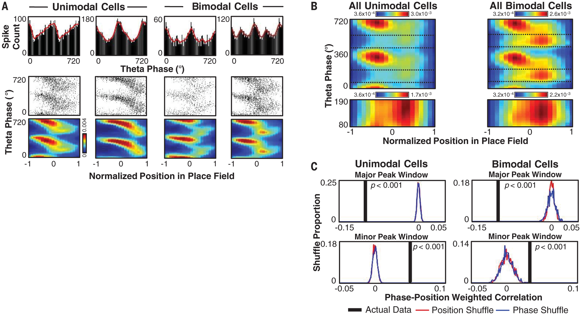
Fig. 3. Phase precession and procession.

(A) Example unimodal and bimodal cells displaying phase precession and/or phase procession. (Top) Spike count per theta phase. (Bottom) Spike plot and smoothed (Gaussian, σ = 2 bins) probability heatmap of theta phase versus normalized location (−1 is entering the field, 1 is leaving). (B) (Top) Smoothed firing probability per theta phase bin (10°) and normalized position in place field bin (0.1), averaged across all cells for open field and linear track sessions. Dotted lines mark major and minor peak boundaries. (Bottom) As in top panel, but showing only the minor peak window with a rescaled colormap. (C) Actual data and distribution of weighted correlation values for 1000 shuffles of position or theta phase in major peak and minor peak windows. The maximum Monte-Carlo P value for either shuffle displayed is noted.
