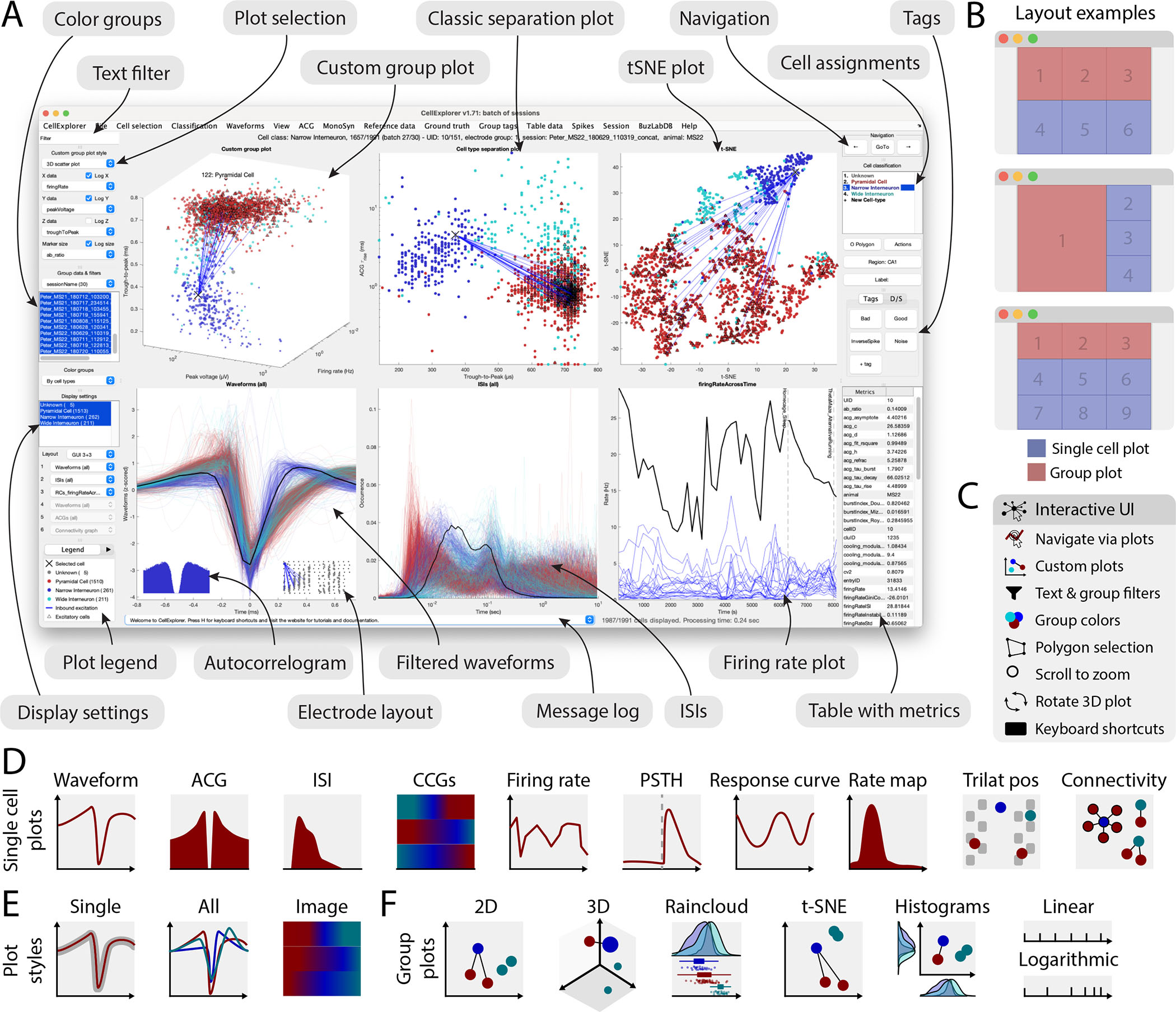
Figure 3: Graphical interface.

A. The interface consists of 4 to 9 main plots, where the top row is dedicated to population-level representations of the neurons. Other plots are selectable and customizable for individual neuron (e.g., single waveforms, ACGs, ISIs, CCGs, PSTHs, response curves, and firing rate maps). The surrounding interface consists of panels placed on either side of the graphs. The left side displays settings and population settings, including a custom plot panel, color group panel, display settings panel, and legends. The right side-panel displays single-cell dimensions, including a navigation panel, neuron assignment panel, tags, and a table with metrics. In addition, there is a text filter and a message log. B. Layout examples highlighting three configurations with 1–3 group plots and 3–6 single neuron plots. C. The interface has many interactive elements, including navigation and selection from plots (left mouse click links to selected cell and right mouse click selects the neuron from all the plots), visualization of monosynaptic connections, various data plotting styles (more than 30+ unique plots built-in), supports custom plots; plotting filters can be applied by text or selection, keyboard shortcuts, zooming any plot by mouse-scrolling and polygon selection of neurons D. Single cell plot options: waveform, Autocorellogram (ACG), Inter-spike-interval (ISI), firing rate across time, Post-Stimulus Time Histogram (PSTH), response curve, spatial firing rate maps, trilaterated neuronal position relative to recording sites, and monosynaptic connectivity graph. E. Most single cell plots have three representations: individual single cell representation, single cell together with the entire population with absolute amplitude and a normalized image representation (colormap). F. Group plotting options: 2D, 3D, raincloud plot, t-SNE, and double histogram. Each dimension can be plotted on linear or logarithmic axes. See also Supplementary Figure 4, 5, 6 and Supplementary Video 1.