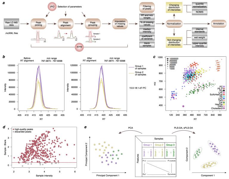
Figure 2.

Schematic illustration of the LC-MS data analysis workflow. (a) Peak picking, alignment, and grouping are followed by the imputation of missing values, filtering, normalization, and annotation of lipid features. IPO and NOMIS abbreviations in the figure correspond to IPO [45,46] and NOMIS [48] tools, respectively. (b) An example of the peak alignment procedure for a deuterium-labeled lipid PC(15:0/18:1). (c) Mass and retention time of lipids with manually verified annotation based on a visually distinguishable ‘grid’ on this scatterplot. (d) A mean-difference plot visualizing the relationship of lipid intensities between biological samples and blank samples. For each peak, the median log10 intensities are calculated among biological samples and among blank samples. Each circle represents the sample intensity and the difference between the sample and blank intensities for a peak. The dashed red line shows the threshold of a two-fold difference between the sample and blank intensities used for peak filtering. (e) An illustrative example of Principal Component Analysis (PCA), Partial Least Squares-Discriminant Analysis (PLS-DA) and sparse PLS-DA score plots. Each data point on both plots corresponds to the coordinates of a single sample in a low-dimensional space.