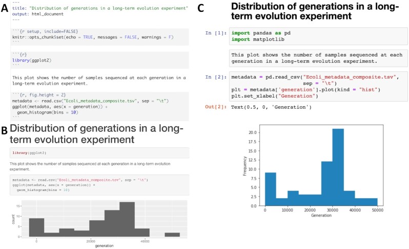
Figure 4:

Examples of computational notebooks. Computational notebooks allow the user to mix text, code, and results in 1 document. A. RMarkdown document viewed in the RStudio integrated development environment; B. rendered HTML file produced by knitting the RMarkdown document [55]. C. Jupyter Notebook, where code, text, and results are rendered inline as each code chunk is executed [56]. The second grey chunk is a raw Markdown chunk with text that will be rendered inline when executed. Both notebooks generate a histogram of a metadata feature, number of generations, from a long-term evolution experiment with Escherichia coli [57]. Computational notebooks facilitate sharing by packaging narrative, code, and visualizations together. Sharing can be enhanced further by packaging computational notebooks with tools like Binder [58]. Binder builds an executable environment (capable of running RStudio and jupyter notebooks) out of a GitHub repository using package management systems and docker to build reproducible and executable software environments as specified in the repository. Binders can be shared with collaborators (or students in a classroom setting), and analysis and visualization can be ephemerally reproduced or altered from the code provided in computational notebooks.