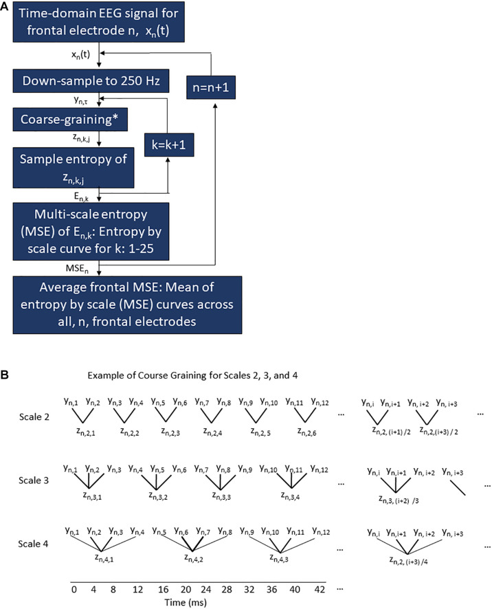
FIGURE 1.

Multi-scale entropy procedure for frontal EEG electrodes (A) and example of course graining (B). (A) A flow chart of the processing algorithm applied to the raw EEG signal for a given condition (pre-operative or intra-operative) for a given subject to generate the frontal average MSE curve for a given condition/subject. The time domain signal recorded at 1,000 Hz from a given frontal electrode, n, is represented as x_n(t) where t ranges from 0 to 3 min. This raw signal x_n(t) is down-sampled to 250 Hz to generate the time series y_n,_τ where τ is the sample number from 1 to 45,000. Each sample encompasses 4 ms. The down-sampled time series y_n,_τ is then course-grained for a given scale k (as shown in the examples of scale k = 2, 3, and 4 in B) to generate the coarse-grained signal z_n,k,j, where z_{n,k = 1,j} at scale 1 is identical to y_n,τ and where j ranges from 1 to (τ + k–1)/k. The sample entropy is then calculated for each z_n,k,j signal to yield an entropy value E_n,k. This is repeated for each scale k. Once E_n,k has been calculated for all scales k = 1–25, an MSE curve for a given subject, condition, and electrode, n. The MSE_n curve ranges on the x-axis from scale k = 1–25. The MSE_n curve on the y-axis is E_n,k. This is repeated for every electrode, n, in the frontal region. Finally, the MSE curves for all n electrodes are averaged across scale k to yield a single frontal MSE curve for each subject/condition. (B) Example of course graining procedure perform on the down-sampled time series for electrode n, y_n,τ, where τ ranges from 1 to 4,500, to yield the course-grained series z_n,k,j where n represents the electrode in question, k is the scale value, and j is the sample number. Scales 2, 3, and 4 are shown for examples above, but this same pattern continues up to scale 25. The temporal resolution associated with the course graining is show on the axis at the bottom of the figure.