Figure 10.

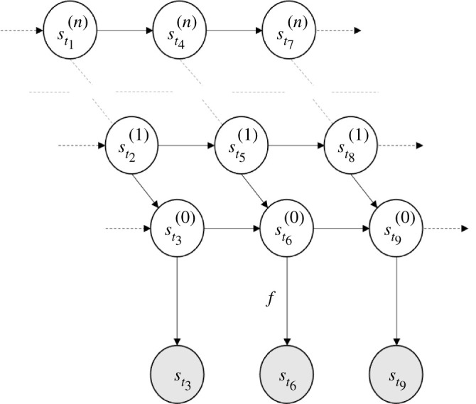
Continuous-time Hidden Markov model. This figure depicts (4.3) in a graphical format, as a Bayesian network [3,31]. The encircled variables are random variables—the processes indexed at an arbitrary sequence of subsequent times $t_1<t_2<\dots <t_9$. The arrows represent relationships of causality. In this hidden Markov model, the (hidden) state process ${\tilde{s}}_t$ is given by an integrator chain—i.e. nested stochastic differential equations $s_t^{(0)},s_t^{(1)},\dots ,s_t^{(n)}$. These processes $s_t^{(i)},i\ge 0$, can, respectively, be seen as encoding the position, velocity, jerk etc, of the process $s_t$.