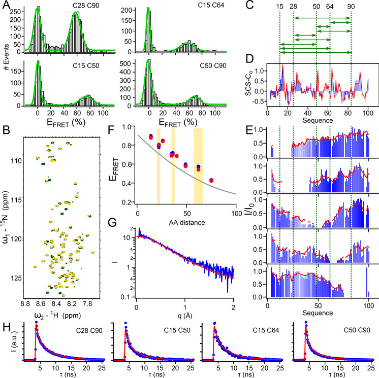
Figure 5.
Description of experimental FRET, PREs, and SAXS by a common multiconformational model. (A) Experimental FRET histograms of P1–100 (black bars) with double Gaussian fit (green) from which EFRET of the nonzero population was extracted. (B) 1H–15N heteronuclear single quantum coherence (HSQC) spectrum of P1–100 C64 unlabeled (green) and labeled with MTSL (yellow). (C) Visualization of FRET distances for which data have been acquired. (D) Cα secondary chemical shifts of P1–100 calculated based on experimental chemical shifts (blue) and based on chemical shifts calculated from an ensemble selected based on five PRE labeling positions, six FRET efficiencies and chemical shifts (red). (E) Experimental (blue) PREs and PREs calculated from the selected ensemble (red). All PREs were used in the selection. PRE labeling sites are indicated by green dashed lines (note that the same cysteines have been used for PRE and FRET labeling). Intensity ratios between the PRE labeled (I) and unlabeled (I0) peaks are shown. (F) FRET efficiencies (EFRET) of P1–100 plotted against the amino acid distance between the fluorophores. The gray line indicates values expected from a flexible-meccano statistical coil (polynomial fit of in silico data presented in Figure 3). Experimental data are shown in blue with error bars resulting from standard deviations calculated from independent measurements. Red points indicate EFRET calculated from the ASTEROIDS selection. Data points plotted in front of a yellow background were not used in the selection. (G) Experimental SAXS curve (blue) and SAXS curve back-calculated from the ASTEROIDS ensemble (red). SAXS data were not used in the selection. (H) Cumulated fluorescence lifetime histograms calculated from the FRET population of the single molecule data (corresponding to FRET mutants shown in (A)). Blue points are experimental data, and red curves are decays back-calculated from the selected ensemble, comprising a scattering contribution and scaled to best fit the experimental data.

